This article investigates the Taylor expansion of the function of t: \exp\left(\frac{1}{2}t^2+xt\right) at t=0. Obviously, this is not difficult; it can be solved by hand or using software. The answer is: 1+x t+\frac{1}{2} \left(x^2+1\right) t^2+\frac{1}{6}\left(x^3+3 x\right) t^3 +\frac{1}{24} \left(x^4+6 x^2+3\right) t^4 + \dots However, this article will present a graphical method I constructed for this series. Through this graphical method, the first few terms of the expansion can be calculated by hand quite intuitively and conveniently. Later, we will discuss the origin of this graphical technique and its further applications.
Graphical Method for the Series: Explanation
First, it is clear that to write out this series, the key is to determine each term of the expansion, which requires finding: f_k (x) = \left.\frac{d^k}{dt^k}\exp\left(\frac{1}{2}t^2+xt\right)\right|_{t=0} f_k (x) is a polynomial in x of degree k with integer coefficients, where k is the order of the expansion and the order of differentiation.
Here, we use a "dot" to represent an x, and a "straight line between two dots" to represent "multiplication". Thus, x^2 can be represented as:
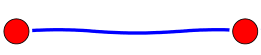
We use the number of "dots" to represent the degree of f_k (x). Every term in f_k (x) should involve k dots. However, f_k (x) is not always of degree k. In such cases, we use "two dots and a wavy line between them" to represent "1." Borrowing a term from physics, we can say these two dots are "coupled" into a constant. Therefore, the following diagram represents the x term in f_3(x):
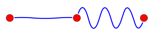
Note that the form of the term is independent of the order in the diagram. That is to say, the following diagram also represents the x term in f_3(x):

To represent the coefficient in front of a term, we add the corresponding number. Thus, the following diagram represents the 3x term in f_3(x):

We also need a restriction: "two wavy lines cannot appear in adjacent positions." That is, the following diagram is forbidden:

Now, it is easy to read the following diagram:
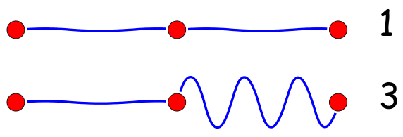
It represents x^3+3x, which is the third-order term of the Taylor expansion. Similarly, the diagram:
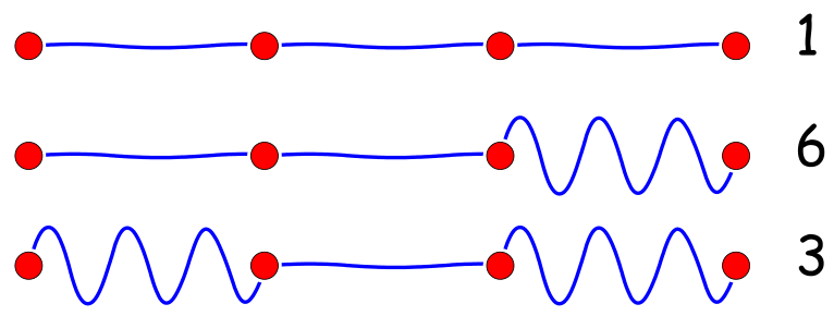
represents x^4+6x^2+3, which is the fourth-order term of the Taylor expansion.
Graphical Method for the Series: Recursion
If this were merely a notation, it would just be another way of writing the series and wouldn’t be very helpful. However, the graphical representation helps us perform recursion intuitively—the process of moving from a k-th order diagram to a (k+1)-th order diagram.
Taking the transition from the 3rd order to the 4th order as an example, the 3rd order diagram is:
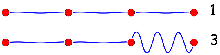
The 4th order diagram has 4 dots, meaning we add 1 dot. We imagine that the added dot emits two types of "signals": a straight-line signal and a wavy-line signal. These two signals probe each dot of the original diagram, but they have different characteristics.
Straight-line Signal
The straight-line signal is "satisfied upon first contact." It has no discrimination between dots; as soon as it detects a dot, it connects to it and stops further probing. Therefore, after probing by the straight-line signal, the 3rd order diagram becomes:
Wavy-line Signal
The wavy-line signal is different from the straight-line signal. It has the ability to identify individual dots and will precisely probe every point where it can be embedded, and then embed itself into them one by one. Therefore, after probing by the wavy-line signal, the 3rd order diagram becomes (where the first three diagrams are equivalent):
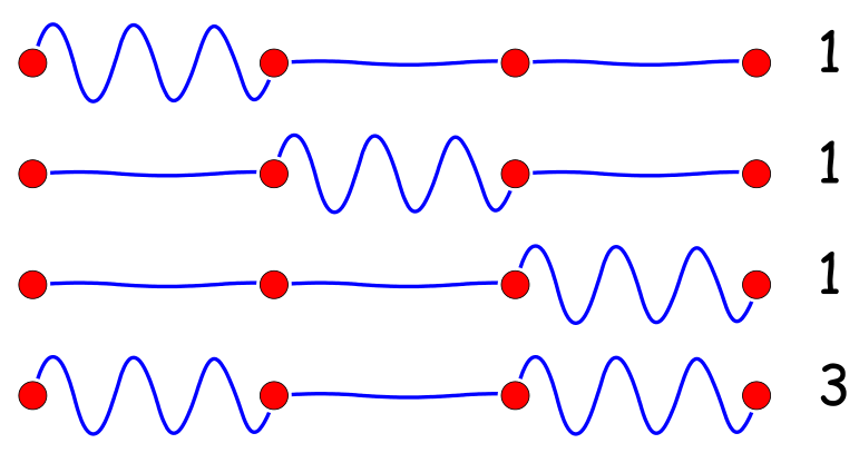
Thus, combining the results of both signals, we obtain the 4th order diagram:
which represents x^4+6x^2+3, the fourth-order term of the Taylor expansion.
This is an example; readers can further simplify the process based on their own understanding.
Graphical Method for the Series: Application
Using the graphical process described above, one can quickly draw the diagrams for the series:
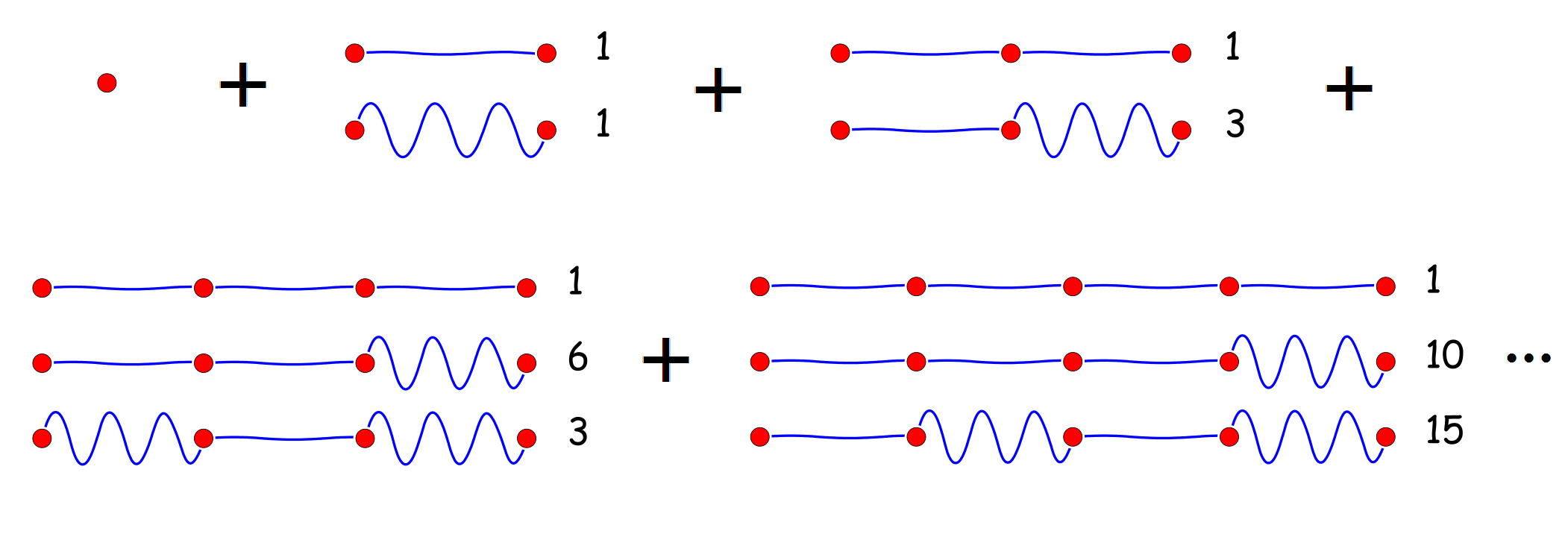
The first term represents f_1 (x) = x, which corresponds to the xt term of the Taylor expansion. The second term represents f_2 (x) = x^2 + 1, which corresponds to the \frac{1}{2!}(x^2 + 1)t^2 term. The third term represents f_3 (x) = x^3 + 3x, which corresponds to the \frac{1}{3!}(x^3 + 3x)t^3 term, and so on. Therefore: \exp\left(\frac{1}{2}t^2+xt\right)=1+x t+\frac{1}{2} \left(x^2+1\right) t^2+\frac{1}{6}\left(x^3+3 x\right) t^3 + \dots
Obviously, if the goal were only to expand this series, the above effort might seem like overkill. However, by changing the meaning of the dots and wavy lines, this method can play a role in much more complex expansions. In fact, I summarized this set of methods while studying "external source techniques" (functional derivatives) in quantum mechanical perturbation theory. There, one is required to calculate: \frac{\delta^n}{\delta x^n}\exp\left[\int \left(xf+\frac{1}{2}fL^{-1}f\right)dt\right] Calculating functional derivatives is far more complex than ordinary derivatives. Therefore, having such a graphical method to assist in the calculation can reduce the computational workload and facilitate the derivation of each term. In fact, in functional derivatives, similar techniques exist; they are equivalent to making each dot a different color to distinguish each term. As one can imagine, the terms would be much more numerous and complex. Of course, I will leave that for future articles.
When reposting, please include the original address of this article: https://kexue.fm/archives/3426
For more detailed information regarding reposting, please refer to: Scientific Space FAQ