Sentiment Analysis of Text (Part II): Deep Learning Models

Deep Learning and Natural Language Processing

In recent years, deep learning algorithms have been applied to the field of natural language processing, achieving superior results compared to traditional models. Scholars such as Bengio built neural probabilistic language models based on deep learning ideas and further utilized various deep neural networks to train language models on large-scale English corpora. This resulted in excellent semantic representations and completed common natural language processing tasks such as syntactic analysis and sentiment classification, providing new ideas for natural language processing in the era of big data.

According to the author’s tests, sentiment analysis models based on deep neural networks often achieve an accuracy of over 95%. The charm and power of deep learning algorithms are evident!

For further information on deep learning, please refer to the following literature:

[1] Yoshua Bengio, Réjean Ducharme, Pascal Vincent, Christian Jauvin. A Neural Probabilistic Language Model, 2003

A New Language Model: http://blog.sciencenet.cn/blog-795431-647334.html

Deep Learning Study Notes: http://blog.csdn.net/zouxy09/article/details/8775360

Deep Learning: http://deeplearning.net

Random Talk on Chinese Automatic Segmentation and Semantic Recognition: http://www.matrix67.com/blog/archives/4212

Application of Deep Learning in Chinese Segmentation and POS Tagging: http://blog.csdn.net/itplus/article/details/13616045

Language Representation

In the article "Chatting: Neural Networks and Deep Learning", the author mentioned that the most important step in the modeling process is feature extraction, and natural language processing is no exception. A core problem in NLP is: how to effectively represent a sentence in numerical form? If this step can be completed, sentence classification becomes straightforward. Obviously, an elementary idea is to assign a unique ID (1, 2, 3, 4...) to each word and treat the sentence as a set of IDs. For example, if 1, 2, 3, 4 represent "I", "you", "love", and "hate", then "I love you" is [1, 3, 2] and "I hate you" is [1, 4, 2]. While this seems effective, it is actually problematic. A stable model might consider 3 and 4 to be very close, so [1, 3, 2] and [1, 4, 2] should yield similar classification results. However, according to our numbering, the words represented by 3 and 4 have completely opposite meanings, so the classification results cannot be the same. Therefore, this encoding method cannot yield good results.

Readers might think: what if I group the IDs of words with similar meanings together (assigning them similar numbers)? Indeed, if there were a way to place similar word IDs together, it would greatly improve the model’s accuracy. But the problem arises: if we give each word a unique ID and set similar words to have similar IDs, we are actually assuming the singularity of semantics—that is, that semantics is only one-dimensional. However, this is not the case; semantics should be multi-dimensional.

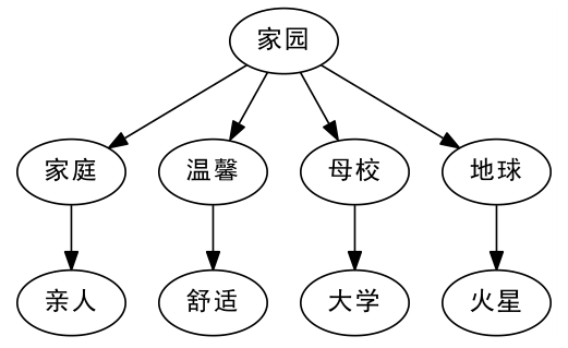
For example, when we talk about "home," some people might think of the synonym "family," and from "family" think of "relatives," all of which are words with similar meanings. On the other hand, from "home," some people might think of "Earth," and from "Earth" think of "Mars." In other words, "relatives" and "Mars" can both be seen as secondary approximations of "home," but there is no obvious connection between "relatives" and "Mars" themselves. Furthermore, semantically speaking, "university" and "comfort" can also be seen as secondary approximations of "home." Clearly, it is difficult to place these words in appropriate positions using only a single unique ID.

Word2Vec: High Dimensions are Here

From the above discussion, we know that the meanings of many words diverge in various directions rather than a single direction, therefore, a unique ID is not ideal. So, how about multiple IDs? In other words, mapping a word to a multi-dimensional vector? Indeed, this is the correct approach.

Why are multi-dimensional vectors feasible? First, multi-dimensional vectors solve the problem of multi-directional divergence; even a two-dimensional vector can rotate 360 degrees, let alone higher dimensions (usually hundreds of dimensions in practical applications). Second, there is a practical advantage: multi-dimensional vectors allow us to represent words using numbers with small variations. How so? We know that in Chinese, the number of words reaches hundreds of thousands. If we give each word a unique ID, the IDs vary from 1 to several hundred thousand. Such a large range makes it difficult to ensure model stability. With high-dimensional vectors, say 20 dimensions, we only need 0s and 1s to represent 2^{20} = 1,048,576 (one million) words. Smaller variations help ensure the stability of the model.

Having said all this, we haven’t yet reached the core point. Now that we have the idea, the question is: how do we place these words into the correct high-dimensional vectors? And importantly, how do we do this without a linguistic background? (In other words, if I want to process an English language task, I don’t need to learn English first; I only need to collect a large number of English articles. How convenient!) We cannot and need not expand further on the principles here, but rather introduce a famous open-source tool from Google based on this idea: Word2Vec.

Simply put, Word2Vec accomplishes what we want: it represents words using high-dimensional vectors (Word Embeddings), places words with similar meanings in close proximity, and uses real-valued vectors (not limited to integers). We only need a large corpus of a certain language to train the model and obtain word vectors. Some benefits of word vectors have been mentioned; they were created to solve the aforementioned problems. Other benefits include: word vectors facilitate clustering, and Euclidean distance or cosine similarity can be used to find words with similar meanings. This effectively solves the "synonym" problem (unfortunately, there doesn’t seem to be a good way to solve the "polysemy" problem yet).

Regarding the mathematical principles of Word2Vec, readers can refer to this series of articles. For the implementation, Google provides the official C source code, which readers can compile themselves. The Gensim library in Python also provides Word2Vec as a sub-library (in fact, this version seems more powerful than the official one).

Representing Sentences: Sentence Vectors

The next problem to solve is: we have segmented the words and converted them into high-dimensional vectors, so a sentence corresponds to a set of word vectors—that is, a matrix, similar to how a digitized image corresponds to a pixel matrix. However, model inputs generally only accept one-dimensional features. What should we do? A simple idea is to flatten the matrix, connecting the word vectors one after another into a longer vector. This idea is possible, but it would make our input dimension as high as several thousand or even tens of thousands, which is difficult to implement in practice. (If tens of thousands of dimensions are not a problem for today’s computers, then for a 1000x1000 image, it would be as high as 1 million dimensions!)

In fact, for image processing, there is already a mature method called Convolutional Neural Networks (CNNs). They are a type of neural network specifically designed to handle matrix inputs, capable of encoding matrix-form inputs into lower-dimensional one-dimensional vectors while retaining most useful information. CNNs can also be directly applied to natural language processing, especially in text sentiment classification, with good results. Related articles include "Deep Convolutional Neural Networks for Sentiment Analysis of Short Texts". However, the principles of sentences differ from images. Directly applying the image processing approach to language, although somewhat successful, feels out of place. Therefore, this is not the mainstream method in natural language processing.

In natural language processing, the methods usually used are Recursive Neural Networks or Recurrent Neural Networks (both called RNNs). Their role is the same as CNNs: encoding matrix-form inputs into lower-dimensional one-dimensional vectors while retaining most useful information. The difference is that CNNs focus more on global fuzzy perception, while RNNs focus on the reconstruction of adjacent positions. Thus, for language tasks, RNNs are more persuasive (language is always composed of adjacent characters forming words, adjacent words forming phrases, adjacent phrases forming sentences, etc.; therefore, it is necessary to effectively integrate or reconstruct information from adjacent positions).

There are endless variations of models. Within the RNNs subset, there are many variants such as ordinary RNNs, GRU, LSTM, etc. Readers can refer to the Keras official documentation: http://keras.io/models/. Keras is a Python deep learning library that provides a large number of deep learning models. Its documentation serves as both a tutorial and a model list.

Building the LSTM Model

After all this discussion, it’s time to do something practical. Now we build a deep learning model for text sentiment classification based on LSTM (Long-Short Term Memory), with the following structure:

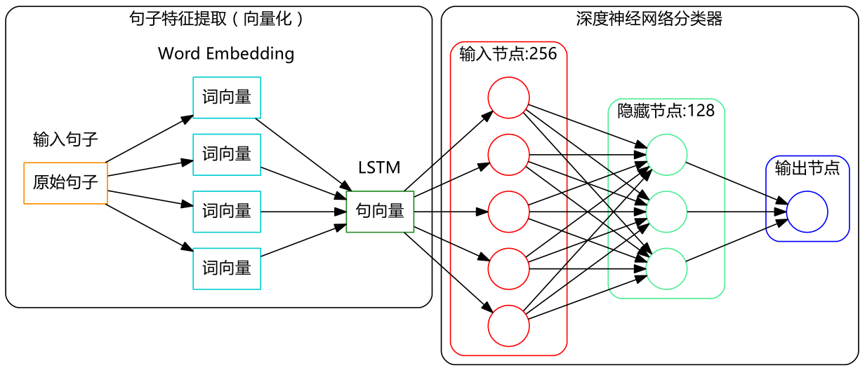
The model structure is simple, and the implementation is easy using Keras, which has already implemented the algorithms for us.

Now let’s talk about two interesting steps.

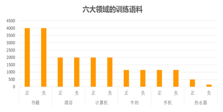
The first step is the collection of labeled corpora. Note that our model is supervised (at least semi-supervised), so we need to collect some categorized sentences—the more, the better. For Chinese text sentiment classification, this step is not easy, as Chinese data is often scarce. When building the model, I pieced together more than 20,000 labeled Chinese sentences (covering six fields) from various channels (online downloads, purchases from Datatang) to train the model.

The second step is the model threshold selection problem. In fact, the predicted result of the training is a continuous real number in the [0, 1] interval. By default, the program sets 0.5 as the threshold—results greater than 0.5 are judged as positive, and those less than 0.5 as negative. This default value is often not the best. As shown below, when studying the impact of different thresholds on the true positive rate and true negative rate, we found a sharp change in the curve within the (0.391, 0.394) interval.

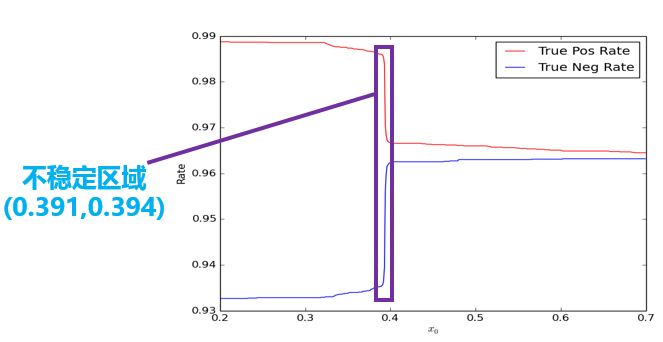
Although in absolute terms it only drops from 0.99 to 0.97, the rate of change is very large. Normally, changes are smooth; a sharp change means something abnormal must have occurred, and the cause is hard to find. In other words, there is an unstable region here, and the prediction results within this region are actually unreliable. Therefore, to be safe, we discard this interval. Only results greater than 0.394 are considered positive, those less than 0.391 are considered negative, and those between 0.391 and 0.394 are left as "undetermined." Experiments show that this approach helps improve the application accuracy of the model.

Summary

This article has roughly introduced the ideas and practical applications of deep learning in text sentiment classification. I am not writing a tutorial on deep learning but rather pointing out the key points. There are many excellent tutorials on deep learning; it is best to read English papers.

Below are my corpus and code. Readers might wonder why I share these "private collections." It’s simple: I’m not in this industry. Data mining is just a hobby for me—a hobby combining mathematics and Python.

Corpus download: sentiment.zip
Collected comment data: sum.zip

Code for building LSTM for text sentiment classification:

import pandas as pd # Import Pandas
import numpy as np # Import Numpy
import jieba # Import Jieba segmentation

from keras.preprocessing import sequence
from keras.optimizers import SGD, RMSprop, Adagrad
from keras.utils import np_utils
from keras.models import Sequential
from keras.layers.core import Dense, Dropout, Activation
from keras.layers.embeddings import Embedding
from keras.layers.recurrent import LSTM, GRU

from __future__ import absolute_import 
from __future__ import print_function

neg=pd.read_excel('neg.xls',header=None,index=None)
pos=pd.read_excel('pos.xls',header=None,index=None) # Reading training corpus
pos['mark']=1
neg['mark']=0 # Labeling training corpus
pn=pd.concat([pos,neg],ignore_index=True) # Merging corpus
neglen=len(neg)
poslen=len(pos) # Counting corpus size

cw = lambda x: list(jieba.cut(x)) # Define segmentation function
pn['words'] = pn[0].apply(cw)

comment = pd.read_excel('sum.xls') # Read comment content
comment = comment[comment['rateContent'].notnull()] # Only read non-empty comments
comment['words'] = comment['rateContent'].apply(cw) # Comment segmentation 

d2v_train = pd.concat([pn['words'], comment['words']], ignore_index = True) 

w = [] # Integrate all words
for i in d2v_train:
    w.extend(i)

dict = pd.DataFrame(pd.Series(w).value_counts()) # Count word frequency
del w,d2v_train
dict['id']=list(range(1,len(dict)+1))

get_sent = lambda x: list(dict['id'][x])
pn['sent'] = pn['words'].apply(get_sent) 

maxlen = 50

print("Pad sequences (samples x time)")
pn['sent'] = list(sequence.pad_sequences(pn['sent'], maxlen=maxlen))

x = np.array(list(pn['sent']))[::2] # Training set
y = np.array(list(pn['mark']))[::2]
xt = np.array(list(pn['sent']))[1::2] # Test set
yt = np.array(list(pn['mark']))[1::2]
xa = np.array(list(pn['sent'])) # Full set
ya = np.array(list(pn['mark']))

print('Build model...')
model = Sequential()
model.add(Embedding(len(dict)+1, 256))
model.add(LSTM(128)) 
model.add(Dropout(0.5))
model.add(Dense(1))
model.add(Activation('sigmoid'))

model.compile(loss='binary_crossentropy', optimizer='adam', metrics=['accuracy'])

model.fit(x, y, batch_size=16, nb_epoch=10) # Training takes several hours

classes = model.predict_classes(xt)
acc = np_utils.accuracy(classes, yt)
print('Test accuracy:', acc)

Please include the original address when reprinting: https://kexue.fm/archives/3414

For more details on reprinting, please refer to: Scientific Space FAQ