Mathieu Equation
In the article "Ponderomotive Force: Stability of the Inverted Pendulum", we analyzed the possibility of stabilizing an inverted pendulum through high-frequency, low-amplitude oscillations and derived the equation of motion: l\ddot{\theta} + [h_0 \omega^2 \cos(\omega t) - g]\sin\theta = 0
This imposes a requirement on the lower bound of the pendulum’s frequency: \omega \gg \sqrt{\frac{g}{h_0}}. However, that lower bound is merely necessary, not sufficient. To fully analyze the motion of this pendulum, the ideal method would be to write the analytical solution for the above ordinary differential equation. Unfortunately, we cannot do this. We can only employ various approximation methods. While approximation methods generally refer to numerical calculation methods, I prefer analytical methods—that is, even for an approximate solution, I hope to find an approximate analytical expression.
First, let us assume \theta \ll 1, so we can use the approximation \sin \theta \approx \theta: l\ddot{\theta} + [h_0 \omega^2 \cos(\omega t) - g]\theta = 0
The above equation is a special type of Mathieu equation. Unlike the Mathieu equations found in standard reference books, where g is negative and h_0 \omega^2 is a small quantity, here h_0 \omega^2 is the dominant term and g is positive. We will adopt a special technique to obtain an approximate analytical solution.
Numerical Analysis
Although I prefer analytical methods, numerical analysis allows us to first glimpse the general nature of the solution. Below is the solution obtained using Matlab for the case l=1, g=10, h=0.01, \omega=500, with initial conditions \theta_0=1, \dot{\theta}_0=0.
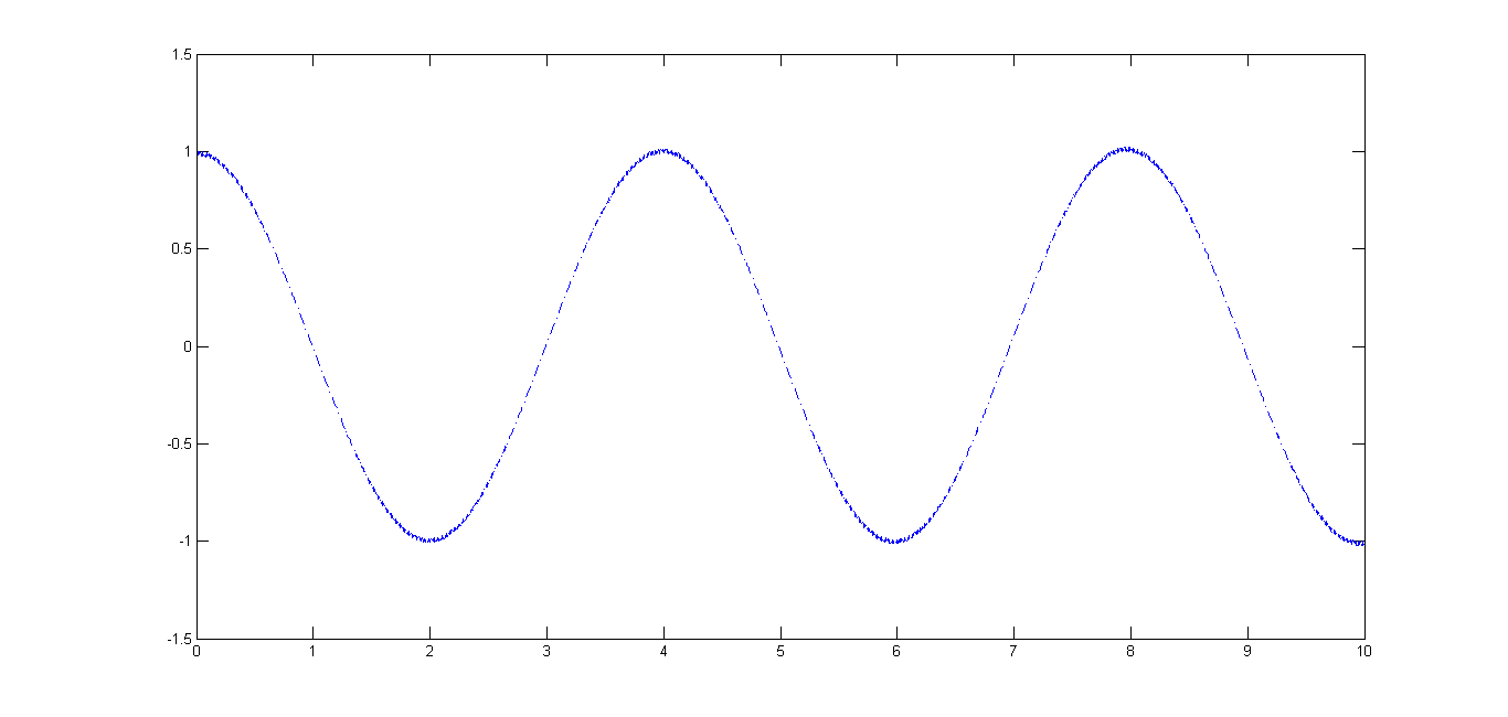
In the case of l=1, g=10, h=0.01, \omega=500, the solution’s graph resembles simple harmonic motion.
The image indicates that the periodic solution is quite ideal, appearing similar to simple harmonic motion. In fact, this is indeed the case. However, let us examine the local behavior more closely.
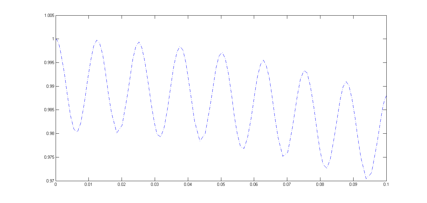
The "simple harmonic motion" shown above is actually superimposed with a high-frequency oscillation.
It is not difficult to see that the actual motion consists of a high-frequency oscillation superimposed on a simple harmonic motion. This explains why solving this problem analytically is difficult, primarily due to the presence of high-frequency functions. For example, \sin \omega t is a very well-behaved function, but if expanded as a Taylor series, it becomes \omega t - \frac{\omega^3 t^3}{6} + \dots; if only the first few terms are taken, the convergence region is extremely small.
The key question now is: since we have observed that the motion is a superposition of two frequencies, can we separate these two frequencies and study them individually? This is the core of this article.
Separation of Frequencies
To separate the frequencies, I have devised the following system of equations: \begin{cases} \ddot{\phi}_1 + \Omega^2 \phi_1 = \varepsilon \left[ \Omega^2 \phi_1 + g(\phi_1 + \phi_2) - (h_0 \omega^2 \cos \omega t) \phi_2 \right] \\ \ddot{\phi}_2 + \omega^2 \phi_2 = \varepsilon \left[ \omega^2 \phi_2 - (h_0 \omega^2 \cos \omega t) \phi_1 \right] \end{cases}
By adding the two equations together and setting \varepsilon=1, we recover the original Mathieu equation, where \theta = \phi_1 + \phi_2, and \Omega is to be determined. The initial conditions are \phi_1(0) = \theta_0, \dot{\phi}_1(0) = 0; \phi_2(0) = h_0 \theta_0, \dot{\phi}_2(0) = 0. This is equivalent to solving the original Mathieu equation under the conditions \theta(0) = (1+h_0)\theta_0, \dot{\theta}(0) = 0.
Treating \varepsilon as a small parameter, we first solve for \phi_2 by neglecting terms containing \varepsilon: \ddot{\phi}_2 + \omega^2 \phi_2 = 0 Combined with the initial conditions, we get: \phi_2 = \theta_0 h_0 \cos \omega t Similarly, applying the same treatment to \phi_1, we find: \phi_1 = \theta_0 \cos \Omega t
To verify the validity of this solution, we must check if the neglected terms are reasonable. For \phi_2, we neglected \varepsilon[\omega^2 \phi_2 - (h_0 \omega^2 \cos \omega t)\phi_1]. Substituting the obtained \phi_1 and \phi_2: \begin{aligned} &\varepsilon[\omega^2 \theta_0 h_0 \cos \omega t - (h_0 \omega^2 \cos \omega t)\theta_0 \cos \Omega t] \\ &= \varepsilon \omega^2 \theta_0 h_0 \cos \omega t (1 - \cos \Omega t) \end{aligned} Since \cos \Omega t is a low-frequency term, it remains approximately 1 over a long period (relative to the period of the high-frequency term). This can be summarized as: in low-frequency terms, high-frequency components average to zero; in high-frequency terms, low-frequency components are treated as constants. Thus, this entire term can be approximately viewed as zero. This indicates that our omission is "self-consistent."
For \phi_1, we neglected \varepsilon[\Omega^2 \phi_1 + g(\phi_1 + \phi_2) - (h_0 \omega^2 \cos \omega t)\phi_2]. Substituting the values gives: \begin{aligned} &\varepsilon \left[ \Omega^2 \theta_0 \cos \Omega t + g(\theta_0 \cos \Omega t + \theta_0 h_0 \cos \omega t) - (h_0 \omega^2 \cos \omega t)\theta_0 h_0 \cos \omega t \right] \\ &= \varepsilon \left[ (\Omega^2 + g)\theta_0 \cos \Omega t - \frac{1}{2}\theta_0 h_0^2 \omega^2 + g \theta_0 h_0 \cos \omega t - \frac{1}{2}\theta_0 h_0^2 \omega^2 \cos 2\omega t \right] \end{aligned} Continuing with our "high-frequency to zero, low-frequency to constant" approach, we obtain: \varepsilon \left[ (\Omega^2 + g)\theta_0 - \frac{1}{2}\theta_0 h_0^2 \omega^2 \right] To make the omission of this term more reasonable, this expression should be approximately zero, therefore: \Omega^2 = \frac{1}{2} h_0^2 \omega^2 - g \geq 0 In the above calculation, we assumed l=1. In the general case, we have: \Omega^2 = \frac{1}{2} h_0^2 \omega^2 - gl \geq 0 This is the same result as derived in Landau’s Mechanics and matches the result by Fan Xiang. Different paths lead to the same result!
Thus, we finally obtain the approximate solution: \theta \approx \theta_0 \cos \Omega t + h_0 \theta_0 \cos \omega t To obtain a higher-precision approximate solution, we could continue expanding the above system of equations in terms of \varepsilon. Due to the complexity of the process, it is omitted here.
When reposting, please include the original address: https://kexue.fm/archives/2471
For more detailed reposting matters, please refer to: Scientific Space FAQ