We usually use a wave equation to describe the vibration of a string. However, the vibration of a string is two-dimensional; that is, its "wave" is a displacement in the vertical direction. Let us consider a one-dimensional ideal spring fixed at one end, with a Hooke’s constant k. Its relaxed state is uniform, its linear density is \rho, its length is l, and its mass is m.
How does it bounce?
We want to analyze the motion of this spring—that is, given the initial state of the spring, we want to see how the density of the spring changes. This situation is similar to a "transverse wave." However, the spring itself is a continuous medium, which we are not familiar with. But we can discretize it, treating it as a spring chain composed of infinitely many small particles, as shown in the figure below:
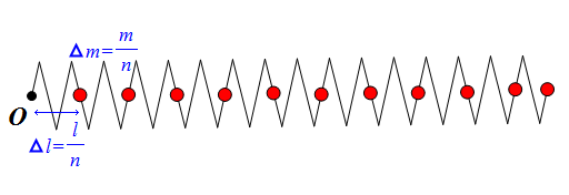
The figure above shows the spring in its relaxed state divided equally into n parts. Assume that the mass of each part \Delta m = \frac{m}{n} is concentrated at the particle on the right end, and every two particles are connected by a spring with length \Delta l = \frac{l}{n}. Since the elastic coefficient is inversely proportional to the length, the elastic coefficient of each small spring is nk. Since this has now become a system of particles, we can analyze it using the usual action. Let the coordinate corresponding to the i-th particle be x_i:
S=\int \left\{\frac{1}{2}\frac{m}{n}\left[\sum_{i=1}^n\left(\frac{dx_i}{dt}\right)^2\right]-\frac{1}{2}nk\left[\sum_{i=1}^n\left(x_i-x_{i-1}-\frac{l}{n}\right)^2\right]\right\}dt
Since \sum_{i=1}^n\left(x_i-x_{i-1}-\frac{l}{n}\right)^2=\sum_{i=1}^n\left[\left(x_i-x_{i-1}\right)^2+\frac{l^2}{n^2}-\frac{2l}{n}\left(x_i-x_{i-1}\right)\right] Because a large number of particles are involved, we only need to calculate the terms containing a large number of particles. In the above expression, the constant term is meaningless, and the final term sums to the difference between the end point and the starting point; this term will not produce a practical effect. Therefore, the effective action is:
S=\int \left\{\frac{m}{2}\frac{1}{n}\left[\sum_{i=1}^n\left(\frac{dx_i}{dt}\right)^2\right]-\frac{k}{2}\frac{1}{n}\left[\sum_{i=1}^n\left(\frac{x_i-x_{i-1}}{1/n}\right)^2\right]\right\}dt
Considering the limit n \to \infty, we find that the above result becomes the familiar definition of a definite integral! Therefore, we first denote x_i as X(i) and introduce a parameter \xi \in [0,1], using \xi instead of n as the label for the particle number, i.e., \xi(i) = \frac{i}{n}. In this way, X(i) can be written as X(\xi). At the same time, it is also a function of time, so X = X(\xi, t). The limit of the above action is:
S=\int \left\{\frac{m}{2}\left[\int_0^1\left(\frac{\partial X}{\partial t}\right)^2d\xi\right]-\frac{k}{2}\left[\int_0^1\left(\frac{\partial X}{\partial \xi}\right)^2 d\xi\right]\right\}dt Rearranging this gives: S=\int dt \int_0^1 d\xi\left[\frac{m}{2}\left(\frac{\partial X}{\partial t}\right)^2-\frac{k}{2}\left(\frac{\partial X}{\partial \xi}\right)^2 \right]
Varying the above action, we obtain the wave equation: m\frac{\partial^2 X}{\partial t^2}=k\frac{\partial^2 X}{\partial \xi^2}
We find that by considering the limit n \to \infty, what was originally a system of ordinary differential equations with infinitely many variables has become a partial differential equation with two variables. This is basic common sense: a partial differential equation is equivalent to a system of infinitely many ordinary differential equations. This is also the fundamental idea of transitioning from particles to field theory. It is no wonder that partial differential equations are difficult; after all, sometimes solving a single ordinary differential equation is not easy. The above equation is formally identical to the general wave equation, only the meaning of the variables has changed. Let’s reconsider the meaning of \xi. In fact, \xi is proportional to the original i, and i is proportional to the mass of the spring from the origin to the i-th particle. That is to say, if X = X(\xi, t), it means that the mass of the section of the spring from the origin to point X is m\xi.
How does it move?
Now we can solve the above equation. This is a basic hyperbolic partial differential equation, and its solution is quite straightforward. We can decompose it as: \left(\frac{\partial}{\partial \xi}-\frac{\partial}{\beta\partial t}\right)\left(\frac{\partial}{\partial \xi}+\frac{\partial}{\beta\partial t}\right)X=0, \quad \beta^2=\frac{k}{m} Applying the transformation u=\xi+\beta t, v=\xi-\beta t, we get: \begin{aligned}2\frac{\partial}{\partial u}=\frac{\partial}{\partial \xi}+\frac{\partial}{\beta\partial t}\\ 2\frac{\partial}{\partial v}=\frac{\partial}{\partial \xi}-\frac{\partial}{\beta\partial t}\end{aligned} The original equation becomes: \frac{\partial^2 X}{\partial u \partial v}=0 Its general solution is: X=F(u)+H(v)=F(\xi+\beta t)+H(\xi-\beta t) where F and H are arbitrary functions. The above represents a general one-dimensional wave. We need to provide the initial state to solve further. Suppose: X|_{t=0}=X_0(\xi), \quad \left.\frac{\partial X}{\partial t}\right|_{t=0}=X_1(\xi) Then we can solve (simply by differentiating the general solution with respect to t and then solving the system): X(\xi,t)=\frac{1}{2}\left[X_0(\xi+\beta t)+X_0(\xi-\beta t)\right]+\frac{1}{2\beta}\int_{\xi-\beta t}^{\xi+\beta t} X_1 (s)ds If it is released from a certain state at rest, then we have: X(\xi,t)=\frac{1}{2}\left[X_0(\xi+\beta t)+X_0(\xi-\beta t)\right]
However, there are some problems with this solution. We will leave the specific analysis and example demonstrations for the next article.
When reprinting, please include the address of this article: https://kexue.fm/archives/2430
For more detailed reprinting matters, please refer to: Scientific Space FAQ