Asymptotic Estimation of the Maximum of $n$ Normal Random Variables

Conclusion First

The basic estimation result for \mathbb{E}[z_{\max}] is:

Let z_1, z_2, \dots, z_n \sim \mathcal{N}(0,1) and z_{\max} = \max\{z_1, z_2, \dots, z_n\}. Then \begin{equation} \mathbb{E}[z_{\max}] \sim \sqrt{2 \log n} \label{eq:E-z-max} \end{equation}

Here, the meaning of \sim in Eq. [eq:E-z-max] is: \begin{equation} \lim_{n \to \infty} \frac{\mathbb{E}[z_{\max}]}{\sqrt{2 \log n}} = 1 \end{equation} It can be seen that as n grows, this result becomes increasingly accurate. A more precise result is: \begin{equation} \mathbb{E}[z_{\max}] \sim \sqrt{2 \log \frac{n}{\sqrt{2\pi}}} \end{equation} We can verify these using Numpy:

import numpy as np

n = 4096
z = np.random.randn(10000, n)
E_z_max = z.max(axis=1).mean()  # $\approx$ 3.63
approx1 = np.sqrt(2 * np.log(n))  # $\approx$ 4.08
approx2 = np.sqrt(2 * np.log(n / np.sqrt(2 * np.pi)))  # $\approx$ 3.85

Fast Upper Bound

For the above conclusion, this article will provide three proofs. The first proof comes from a response by @Sivaraman in the thread "Expectation of the maximum of gaussian random variables". It actually only proves \mathbb{E}[z_{\max}] \leq \sqrt{2 \log n}, but the proof process is quite brilliant and worth learning.

The proof cleverly utilizes the convexity of \exp: for any t > 0, we can write \begin{equation} \exp(t\mathbb{E}[z_{\max}]) \leq \mathbb{E}[\exp(t z_{\max})] = \mathbb{E}[\max_i \exp(t z_i)] \leq \sum_{i=1}^n \mathbb{E}[\exp(t z_i)] = n \exp(t^2 / 2) \end{equation} The first \leq is based on Jensen’s inequality, and the second \leq replaces the maximum with a summation. Now, taking the logarithm of both sides and rearranging gives \begin{equation} \mathbb{E}[z_{\max}] \leq \frac{\log n}{t} + \frac{t}{2} \end{equation} Note that this holds for any t > 0, so we can choose the t that minimizes the right-hand side to achieve the highest degree of approximation. From basic inequalities, the minimum of the right-hand side is reached at t = \sqrt{2 \log n}. Substituting this back gives \begin{equation} \mathbb{E}[z_{\max}] \leq \sqrt{2 \log n} \end{equation} The characteristic of this derivation is that it is simple and fast, requiring little additional prior knowledge. Although it is theoretically only an upper bound, it is surprisingly accurate and happens to be the asymptotic result.

Conventional Approach

For those accustomed to step-by-step formula derivation (like the author), the above derivation might feel a bit like a "shortcut." The conventional solution should involve first finding the probability density function of z_{\max} and then calculating the expectation through integration. In this section, we follow this approach.

Probability Density

For a 1D distribution, the probability density function (PDF) and the cumulative distribution function (CDF) are two sides of the same coin. Finding the PDF of z_{\max} requires the CDF as an auxiliary step. The PDF of the standard normal distribution is p(z) = \exp(-z^2/2)/\sqrt{2\pi}, and the CDF \Phi(z) = \int_{-\infty}^z p(x)dx is a non-elementary function representing the probability that a random variable is less than or equal to z.

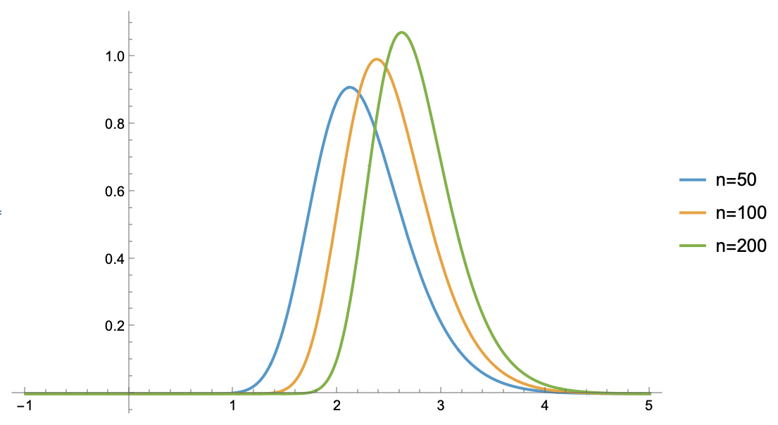
To find the CDF of z_{\max}, i.e., P(z_{\max} \leq z), it is easy to see that z_{\max} \leq z is equivalent to z_1 \leq z, z_2 \leq z, \dots, z_n \leq z holding simultaneously. Since z_i are sampled independently, the probability of them holding simultaneously is the product of their individual probabilities: \begin{equation} P(z_{\max} \leq z) = \prod_{i=1}^n P(z_i \leq z) = [\Phi(z)]^n \end{equation} Thus, the CDF of z_{\max} is [\Phi(z)]^n, a very concise result. Note that we haven’t used the condition that z follows a normal distribution yet, so this is actually a general result: for n numbers sampled i.i.d. from any distribution, the CDF of their maximum is the n-th power of the original distribution’s CDF. Now, differentiating it gives the PDF of z_{\max}, denoted as p_{\max}(z): \begin{equation} p_{\max}(z) = n[\Phi(z)]^{n-1} p(z) \end{equation}

The plots of p_{\max}(z) for n=50, 100, 200 are shown below:

Inverse Transform Sampling

The final proof is based on the idea of inverse transform sampling: let the CDF of a 1D distribution be \Phi(z) and its inverse function be \Phi^{-1}(z). Then, a way to sample from this distribution is: \begin{equation} z = \Phi^{-1}(\varepsilon), \qquad \varepsilon \sim U(0,1) \end{equation} That is, the inverse CDF can transform a uniform distribution into the target distribution. Thus, sampling n points z_1, z_2, \dots, z_n from the target distribution is equivalent to saying that \Phi(z_1), \Phi(z_2), \dots, \Phi(z_n) are n points sampled from U(0,1). To find \mathbb{E}[z_{\max}], we can approximately assume: \begin{equation} \mathbb{E}[z_{\max}] \approx \Phi^{-1}(\mathbb{E}[\Phi(z_{\max})]) \end{equation} This means we first find the corresponding expectation in U(0,1) and then transform it back via \Phi^{-1}. It is easy to guess that for n points sampled from U(0,1), the average value of their maximum is approximately \frac{n}{n+1} (dividing the interval (0,1) into n+1 equal parts, there are n points inside, and we take the largest one). Thus, \mathbb{E}[z_{\max}] \approx \Phi^{-1}(\frac{n}{n+1}). This is a general result; next, we combine it with the specific CDF to get a more explicit solution.

For the standard normal distribution, we have \Phi(z) = \frac{1}{2} + \frac{1}{2}\mathop{\mathrm{erf}}\left(\frac{z}{\sqrt{2}}\right) = 1 - \frac{1}{2}\mathop{\mathrm{erfc}}\left(\frac{z}{\sqrt{2}}\right). The Erfc function has an asymptotic form \mathop{\mathrm{erfc}}(z) \sim \frac{\exp(-z^2)}{z\sqrt{\pi}} (which can be derived via integration by parts). Substituting this into \Phi(z) gives: \begin{equation} \Phi(z) \sim 1 - \frac{\exp(-z^2/2)}{z\sqrt{2\pi}} \end{equation} Thus, finding \Phi^{-1}(\frac{n}{n+1}) is roughly equivalent to solving the equation: \begin{equation} \frac{\exp(-z^2/2)}{z\sqrt{2\pi}} = \frac{1}{n+1} \end{equation} This equation is very similar to the one in the previous section. Following the same solving process, we obtain: \begin{equation} \mathbb{E}[z_{\max}] \sim \sqrt{2\log\frac{n+1}{\sqrt{2\pi}}} \sim \sqrt{2\log\frac{n}{\sqrt{2\pi}}} \sim \sqrt{2\log n} \end{equation}

Application Example

In the article "Low-precision Attention May Have Biased Rounding Errors", we introduced a mechanism where low-precision Attention produces calculation bias. One condition for this is the simultaneous existence of multiple maximum values in the same row of Attention Logits. Is this condition easily satisfied? Using the results of this article, we can estimate the probability of its occurrence.

Suppose a row has n Logits, all sampled i.i.d. from \mathcal{N}(0,1). We could consider general mean and variance, but it doesn’t change the subsequent conclusion. Of course, the actual situation might not be a normal distribution, but this serves as a good baseline. The question is: if we convert these n Logits to BF16 format, what is the probability that at least two identical maximum values appear?

According to the previous results, the maximum of these n Logits is approximately \nu = \sqrt{2\log\frac{n-1}{\sqrt{2\pi}}}. Since BF16 has only 7 bits of mantissa, its relative precision is 2^{-7} = 1/128. As long as any of the remaining n-1 Logits falls into the interval (\frac{127}{128}\nu, \nu], we can consider that two identical maximum values have appeared under BF16. Based on the meaning of the PDF, the probability of a single sample falling into this interval is p(\nu)\frac{\nu}{128}. Then, the probability that at least one of the n-1 numbers falls into this interval is: \begin{equation} 1 - \left(1 - p(\nu)\frac{\nu}{128}\right)^{n-1} = 1 - \left(1 - \frac{\nu/128}{n-1}\right)^{n-1} \approx 1 - e^{-\nu/128} \approx \frac{\nu}{128} \end{equation} Note that once we have fixed the maximum value, the remaining n-1 numbers are technically no longer i.i.d. from the standard normal distribution. However, calculating it as i.i.d. still provides a simple approximation that the author believes is usable when n is large enough.

Comparison with numerical simulation results:

import jax
import jax.numpy as jnp

def proba_of_multi_max(n, T=100, seed=42):
    p, key = 0, jax.random.key(seed)
    for i in range(T):
        key, subkey = jax.random.split(key)
        logits = jax.random.normal(subkey, (10000, n)).astype('bfloat16')
        p += ((logits == logits.max(axis=1, keepdims=True)).sum(axis=1) > 1).mean()
    return p / T

def approx_result(n):
    return jnp.sqrt(2 * jnp.log(n / jnp.sqrt(2 * jnp.pi))) / 128

# n=128: proba $\approx$ 0.0182, approx $\approx$ 0.0219
# n=4096: proba $\approx$ 0.0283, approx $\approx$ 0.0301
# n=65536: proba $\approx$ 0.0530, approx $\approx$ 0.0352

As we can see, even with a sequence length of only 128, there is about a 2% probability of duplicate maximums. This is significant because Flash Attention is computed in blocks, and a typical block length is 128. If the probability for every 128 Logits is 2%, then the probability of at least one duplicate maximum occurring during the Attention calculation of the entire sample is on the order of 1 - 0.98^{n^2/128} (remember the Logits matrix size is the square of the sequence length). For n=4096, this is already close to 100%.

There is a small detail: in actual Attention calculations, the Logits matrix is usually not in BF16 format directly; instead, it is converted to BF16 after subtracting the \max and applying \exp. In this case, the maximum value is 1, and the problem is equivalent to the probability of at least two 1s appearing in each row of the matrix. However, the results of this detailed version will not differ significantly from directly converting the Logits matrix to BF16.

Summary

In this article, we estimated the mathematical expectation of the maximum of n normal random variables using three different methods and used the results to provide a simple estimate of the probability of duplicate maximums appearing in low-precision Attention matrices.

Original Address: https://kexue.fm/archives/11390

For more details on reprinting, please refer to: "Scientific Space FAQ"