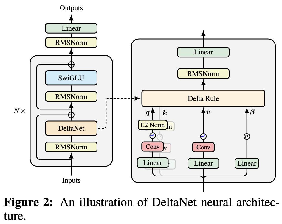
If you have been following developments in model architectures, you will notice that newer Linear Attention models (refer to A Brief History of Linear Attention: From Imitation and Innovation to Feedback) have added "Short Conv" to \boldsymbol{Q}, \boldsymbol{K}, \boldsymbol{V}. An example is DeltaNet, as shown in the figure below:
Why add this Short Conv? An intuitive understanding might be to increase model depth, enhance the model’s Token-Mixing capability, etc. Simply put, it is to compensate for the decline in expressive power caused by linearization. While this explanation is generally correct, it belongs to the category of "universal template" answers. We want to have a more accurate understanding of its actual mechanism.
Next, I will provide my own understanding (or more accurately, a conjecture).
Test-Time Training
From A Brief History of Linear Attention: From Imitation and Innovation to Feedback, we know that the core idea behind current modern Linear Attention is TTT (Test-Time Training) or Online Learning. TTT is based on the similarity between optimizer updates and RNN iterations. It constructs (not necessarily linear) RNN models through an optimizer. Linear Attention variants such as DeltaNet, GDN, and Comba can all be seen as special cases of this.
Specifically, TTT treats \boldsymbol{K}, \boldsymbol{V} as pairs of corpus data (\boldsymbol{k}_1, \boldsymbol{v}_1), (\boldsymbol{k}_2, \boldsymbol{v}_2), \dots, (\boldsymbol{k}_t, \boldsymbol{v}_t). We use them to train a model \boldsymbol{v} = \boldsymbol{f}(\boldsymbol{S}_t; \boldsymbol{k}), and then output \boldsymbol{o}_t = \boldsymbol{f}(\boldsymbol{S}_t; \boldsymbol{q}_t), where \boldsymbol{S}_t represents the model parameters updated via SGD: \boldsymbol{S}_t = \boldsymbol{S}_{t-1} - \eta_t \nabla_{\boldsymbol{S}_{t-1}} \mathcal{L}(\boldsymbol{f}(\boldsymbol{S}_{t-1}; \boldsymbol{k}_t), \boldsymbol{v}_t) Of course, if we wish, we can consider other optimizers. For example, Test-Time Training Done Right experimented with the Muon optimizer. Besides changing the optimizer, one can also flexibly change the architecture of the model \boldsymbol{v} = \boldsymbol{f}(\boldsymbol{S}_t; \boldsymbol{k}) and the loss function \mathcal{L}(\boldsymbol{f}(\boldsymbol{S}_{t-1}; \boldsymbol{k}_t), \boldsymbol{v}_t). Furthermore, we can consider Mini-batch TTT based on chunks.
It is not hard to imagine that, theoretically, TTT is highly flexible and can construct arbitrarily complex RNN models. When the architecture choice is a linear model \boldsymbol{v} = \boldsymbol{S}_t \boldsymbol{k} and the loss function is mean squared error, the result corresponds to DeltaNet; if we add some regularization terms, variants like GDN can be derived.
A Soul-Searching Question
Putting TTT at the forefront is mainly to show that the underlying logic of current mainstream Linear Attention is the same as TTT: the core is Online Learning on corpus pairs (\boldsymbol{k}_1, \boldsymbol{v}_1), (\boldsymbol{k}_2, \boldsymbol{v}_2), \dots, (\boldsymbol{k}_t, \boldsymbol{v}_t). This naturally leads to a question: Why do this? What exactly is being learned?
To answer this, we first need to reflect on "what we actually want." According to the characteristics of Softmax Attention, what we want is to calculate an \boldsymbol{o}_t based on (\boldsymbol{k}_1, \boldsymbol{v}_1), \dots, (\boldsymbol{k}_t, \boldsymbol{v}_t) and \boldsymbol{q}_t. Ideally, this process should depend on all (\boldsymbol{k}, \boldsymbol{v}) pairs. At the same time, we hope to achieve this goal with constant complexity. Thus, an intuitive idea is to first compress (\boldsymbol{k}, \boldsymbol{v}) into a fixed-size State (independent of t) and then read from this State.
How is this compression achieved? The TTT idea is: design a model \boldsymbol{v} = \boldsymbol{f}(\boldsymbol{S}_t; \boldsymbol{k}), and then use these (\boldsymbol{k}, \boldsymbol{v}) pairs to "train" the model. Once training is complete, the model in some sense "memorizes" these (\boldsymbol{k}, \boldsymbol{v}) pairs. This is equivalent to compressing all (\boldsymbol{k}, \boldsymbol{v}) into the fixed-size model weights \boldsymbol{S}_t. As for how \boldsymbol{q}_t utilizes \boldsymbol{S}_t, substituting it directly into the model to get \boldsymbol{o}_t = \boldsymbol{f}(\boldsymbol{S}_t; \boldsymbol{q}_t) is a natural choice, though in principle, we could design other ways to utilize it.
In other words, the core task of TTT is to utilize the fact that "training a model" is approximately equal to "memorizing the training set" to achieve the compression of \boldsymbol{K} and \boldsymbol{V}. However, the fact that "training a model" is approximately equal to "memorizing the training set" is not trivial; it requires certain preconditions.
Key-Value Homology
For example, if we set \boldsymbol{K}=\boldsymbol{V}, the TTT framework theoretically fails because the optimal solution for the model \boldsymbol{v} = \boldsymbol{f}(\boldsymbol{S}_t; \boldsymbol{k}) would be the identity transformation. This is a trivial solution, meaning nothing was memorized. Models with online updates like DeltaNet might still be salvageable, but models based on exact solutions like MesaNet would simply output the identity matrix \boldsymbol{I}.
Some readers might ask: why would anyone consider the unscientific choice of \boldsymbol{K}=\boldsymbol{V}? Indeed, \boldsymbol{K}=\boldsymbol{V} is an extreme case, used here only as an example to show that "training a model" \approx "memorizing the training set" does not hold arbitrarily. Secondly, we have already verified in The Road to Transformer Upgrade: 20. Why is MLA Good? (Part 1) that for Softmax Attention, \boldsymbol{K}=\boldsymbol{V} can still yield decent results.
This indicates that \boldsymbol{K}=\boldsymbol{V} is not an inherent obstacle for the Attention mechanism, but it can cause model failure within the TTT framework. This is because when \boldsymbol{K} and \boldsymbol{V} overlap completely, there is nothing to learn in the regression between them. Similarly, we can imagine that the higher the information overlap between \boldsymbol{K} and \boldsymbol{V}, the less there is to learn, and consequently, the lower the degree of "training set" memorization by TTT.
In general Attention mechanisms, \boldsymbol{q}_t, \boldsymbol{k}_t, \boldsymbol{v}_t are all obtained from the same input \boldsymbol{x}_t through different linear projections. In other words, \boldsymbol{k}_t and \boldsymbol{v}_t share the same source \boldsymbol{x}_t, which always creates a sense of "predicting oneself," limiting what can be learned.
Convolution to the Rescue
How can we make TTT learn more valuable results when keys and values are homologous or even when \boldsymbol{K}=\boldsymbol{V}? Actually, the answer has existed for a long time—traceable back to Word2Vec or even earlier—which is: do not "predict yourself," but "predict the surroundings."
Taking Word2Vec as an example, we know its training method is "center word predicts context." The previously popular BERT used MLM for pre-training, where certain words are masked to be predicted, which can be described as "context predicts center word." Current mainstream LLMs use NTP (Next Token Prediction) as the training task, predicting the next word based on the preceding text. Clearly, their common feature is not predicting oneself, but predicting the surroundings.
Therefore, to improve TTT, one must change the "predicting oneself" pairing method of (\boldsymbol{k}_t, \boldsymbol{v}_t). Considering that current LLMs are primarily based on NTP, we can also consider NTP in TTT, such as using (\boldsymbol{k}_{t-1}, \boldsymbol{v}_t) to construct corpus pairs—that is, using \boldsymbol{k}_{t-1} to predict \boldsymbol{v}_t. This way, even if \boldsymbol{K}=\boldsymbol{V}, a non-trivial result can be learned. At this point, both the internal and external tasks of TTT are NTP, providing a beautiful consistency.
However, using only \boldsymbol{k}_{t-1} to predict \boldsymbol{v}_t seems to waste \boldsymbol{k}_t. So, a further idea is to
mix \boldsymbol{k}_{t-1} and \boldsymbol{k}_t in some way before
predicting \boldsymbol{v}_t. By now,
you might have realized: "mixing \boldsymbol{k}_{t-1} and \boldsymbol{k}_t in some way" is exactly what
a Conv with kernel_size=2 does! Thus, adding Short Conv to
\boldsymbol{K} transforms the TTT
training objective from "predicting oneself" to NTP, giving TTT at least
the ability to learn an n-gram model.
As for adding Short Conv to \boldsymbol{Q} and \boldsymbol{V}, it is largely incidental. According to information from the FLA (Flash Linear Attention) group, while adding it to \boldsymbol{Q} and \boldsymbol{V} has some effect, it is far less significant than the improvement brought by adding Short Conv to \boldsymbol{K}. This serves as further evidence for our conjecture.
Summary
This article provides a self-derived understanding of the question "Why do Linear Attention models add Short Conv?"
Reprinting should include the original address of this article: https://kexue.fm/archives/11320
For more detailed reprinting matters, please refer to: Scientific Space FAQ