Equioscillation Theorem: Necessary and Sufficient Conditions for Optimal Polynomial Approximation

Equioscillation

Let us first present the conclusion:

Equioscillation Theorem Let f(x) be a polynomial of degree at most n, and g(x) be a continuous function on the interval [a,b]. Then \begin{equation} f^* = \mathop{\mathrm{arg\,min}}_f \max_{x\in[a,b]} |f(x) - g(x)| \end{equation} if and only if there exist a\leq x_0 < x_1 < \cdots < x_{n+1} \leq b and \sigma\in\{0,1\} such that \begin{equation} f^*(x_k) - g(x_k) = (-1)^{k+\sigma} \max_{x\in[a,b]} |f^*(x) - g(x)| \end{equation}

The Equioscillation Theorem is sometimes directly called “Chebyshev’s Theorem” because it was first discovered by Chebyshev. Although the textual description of the theorem seems complex, it actually has a very intuitive geometric meaning, as shown in the figure below:

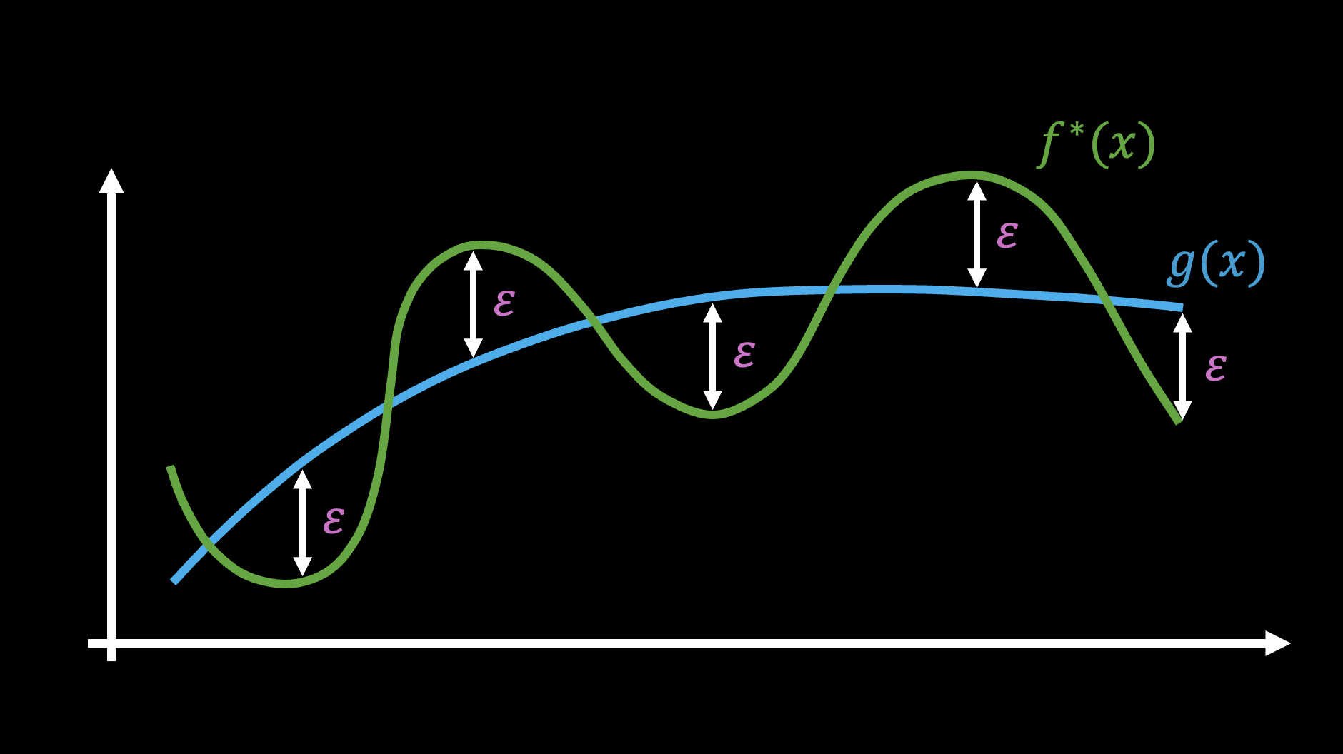
Simply put, the best n-th order polynomial approximation of a function must cross the original function in an alternating fashion. This is very intuitive, but the Equioscillation Theorem tells us that there are “at least n+2 alternating occurrences of the maximum error,” which is a very strong quantitative signal.

The Idea of Differentiation

The error metric used in the Equioscillation Theorem is \max_{x\in[a,b]} |f(x) - g(x)|, which aims to minimize the maximum error. Its advantage is that it automatically focuses on the areas with the largest error without requiring extra hyperparameters to tune.

We know that the standard method for finding an extremum is to take the derivative and set it to zero. However, differentiating a metric involving \max is not trivial. Note that we have: \begin{equation} \max_{x\in[a,b]} |f(x) - g(x)| = \lim_{p\to\infty} \left(\int_a^b |f(x)-g(x)|^p dx\right)^{1/p} = \Vert f(x)-g(x)\Vert_{\infty} \end{equation} That is, it is the infinite version of the L_p norm. If p is a finite number, the derivative can be calculated directly according to standard formulas, but as p\to\infty, new changes may occur. In this case, the safest way is to return to the original definition of the derivative: \begin{equation} \mathcal{D}_x[h(x),u] = \lim_{\epsilon\to 0} \frac{h(x + \epsilon u) - h(x)}{\epsilon} \end{equation} If the limit exists and can be expressed in the form of an inner product \langle \varphi(x),u\rangle, then \varphi(x) is the derivative (gradient) of h(x). If h(x) reaches its minimum at x, then for a sufficiently small non-zero \epsilon, it must hold that h(x + \epsilon u) \geq h(x). If this inequality holds for any u, then it must be that \varphi(x)=0. This is the principle of finding the extremum by setting the derivative to zero.

A Simple Example

Let’s start with a simple example. Define h(x_1,x_2) = \max(x_1,x_2) and consider the one-sided limit: \begin{equation} \mathcal{D}_{(x_1,x_2)}[h(x_1,x_2),(u_1,u_2)] = \lim_{\epsilon\to 0^+} \frac{\max(x_1 + \epsilon u_1,x_2 + \epsilon u_2) - \max(x_1,x_2)}{\epsilon} \end{equation}

Next, we discuss by cases. The first case is x_1 > x_2. Since we are considering the limit as \epsilon is sufficiently small, when x_1 \neq x_2, the added \epsilon u_1, \epsilon u_2 are not enough to change the ordering, i.e., x_1 + \epsilon u_1 > x_2 + \epsilon u_2. Therefore: \begin{equation} \mathcal{D}_{(x_1,x_2)}[h(x_1,x_2),(u_1,u_2)] = \lim_{\epsilon\to 0^+} \frac{(x_1 + \epsilon u_1) - x_1}{\epsilon} = u_1 \end{equation} Similarly, when x_1 < x_2, we have: \begin{equation} \mathcal{D}_{(x_1,x_2)}[h(x_1,x_2),(u_1,u_2)] = \lim_{\epsilon\to 0^+} \frac{(x_2 + \epsilon u_2) - x_2}{\epsilon} = u_2 \end{equation} Finally, when x_1=x_2, we have \max(x_1 + \epsilon u_1,x_2 + \epsilon u_2)=x_1 + \epsilon \max(u_1, u_2), so: \begin{equation} \mathcal{D}_{(x_1,x_2)}[h(x_1,x_2),(u_1,u_2)] = \lim_{\epsilon\to 0^+} \frac{(x_1 + \epsilon \max(u_1, u_2)) - x_1}{\epsilon} = \max(u_1,u_2) \end{equation} This can be similarly generalized to \bm{x}=(x_1,\cdots,x_n) and \bm{u}=(u_1,\cdots,u_n). By careful observation, one can find the rule is “first find the positions where \bm{x} reaches its maximum value, and then find the maximum value among the corresponding components of \bm{u},” i.e., \begin{equation} \mathcal{D}_{\bm{x}}[\max(\bm{x}),\bm{u}] = \lim_{\epsilon\to 0^+} \frac{\max(\bm{x} + \epsilon \bm{u}) - \max(\bm{x})}{\epsilon} = \max_{i\in\mathop{\mathrm{arg\,max}}(\bm{x})} u_i \end{equation} Here, we do not exclude the possibility that the maximum value of \bm{x} occurs at multiple positions, so \mathop{\mathrm{arg\,max}}(\bm{x}) is a set.

It is not difficult to see that the above expression cannot be written in the form \langle \bm{\varphi}(\bm{x}),\bm{u}\rangle, which means that the \max operator does not have a gradient in the strict sense. Of course, the probability of two numbers being exactly equal is small, so if we assume there is only one position for the maximum value, the gradient can be isolated, resulting in \mathop{\mathrm{onehot}}(\mathop{\mathrm{arg\,max}}(\bm{x})). This is exactly how the \max operator is implemented in deep learning frameworks.

Adding Absolute Values

Let |\bm{x}| be the new vector obtained by taking the absolute value of each component of \bm{x}. Now we consider the derivative of \max(|\bm{x}|). Note that we have: \begin{equation} \max(|\bm{x}|) = \max((-\bm{x}, \bm{x})) \end{equation} where (-\bm{x}, \bm{x}) represents the concatenation of the two vectors into a new vector. After removing the absolute value, we can directly substitute the result from the previous section: \begin{equation} \mathcal{D}_{\bm{x}}[\max(|\bm{x}|),\bm{u}] = \mathcal{D}_{(-\bm{x},\bm{x})}[\max((-\bm{x},\bm{x})),(-\bm{u},\bm{u})] = \max_{i\in\mathop{\mathrm{arg\,max}}((-\bm{x},\bm{x}))} (-\bm{u},\bm{u})_i \end{equation} This can be further simplified. Note that when x_i\neq 0, at most one of \pm x_i can be the maximum. If x_i is the maximum, it must be positive, and the value participating in the sorting is u_i; conversely, if -x_i is the maximum, x_i is negative, and the value participating in the sorting is -u_i. Thus, we have: \begin{equation} \mathcal{D}_{\bm{x}}[\max(|\bm{x}|),\bm{u}] = \max_{i\in\mathop{\mathrm{arg\,max}}(|\bm{x}|)} \mathop{\mathrm{sign}}(x_i) u_i \end{equation} Which can also be written as: \begin{equation} \mathcal{D}_{\bm{x}}[\Vert\bm{x}\Vert_{\infty},\bm{u}] = \max_{i\in\mathop{\mathrm{arg\,max}}(|\bm{x}|)} \mathop{\mathrm{sign}}(x_i) u_i \end{equation} This holds provided that \bm{x}\neq \bm{0}. It can be generalized to functions on a closed interval: for all f,g\in \mathcal{C}[a,b], f\neq 0, we have: \begin{equation} \mathcal{D}_f[\Vert f\Vert_{\infty},g] = \max_{x\in\mathop{\mathrm{arg\,max}}(|f(x)|)} \mathop{\mathrm{sign}}(f(x)) g(x) \end{equation} This is the key derivative equation needed to prove the Equioscillation Theorem. It is worth noting that in the proof process of these two sections, we actually only used case-by-case discussion without any approximation. Therefore, we can find a sufficiently small threshold \tau such that for all \epsilon\in[0,\tau], the following holds: \begin{equation} \Vert f + \epsilon g\Vert_{\infty} = \Vert f\Vert_{\infty} + \epsilon\, \mathcal{D}_f[\Vert f\Vert_{\infty},g] = \Vert f\Vert_{\infty} + \epsilon\max_{x\in\mathop{\mathrm{arg\,max}}(|f(x)|)} \mathop{\mathrm{sign}}(f(x)) g(x) \label{eq:eps-x} \end{equation}

Necessary and Sufficient Conditions

This section formally begins the discussion of optimal approximation. We first prove a more general result than polynomial approximation, which is attributed to Kolmogorov:

Kolmogorov Theorem Let \mathcal{S}\subseteq \mathcal{C}[a,b] be a linear subspace of \mathcal{C}[a,b], f^*\in \mathcal{S} and g\in \mathcal{C}[a,b]. Then \begin{equation} f^* = \mathop{\mathrm{arg\,min}}_f \Vert f - g\Vert_{\infty} = \mathop{\mathrm{arg\,min}}_f \max_{x\in[a,b]} |f(x) - g(x)| \end{equation} if and only if for any h\in \mathcal{S}, it holds that \begin{equation} \mathcal{D}_{f^*}[\Vert f^* - g\Vert_{\infty}, h] = \max_{x\in\mathop{\mathrm{arg\,max}}(|f^*(x) - g(x)|)} \mathop{\mathrm{sign}}(f^*(x) - g(x)) h(x) \geq 0\label{eq:cond-1} \end{equation}

The proof consists of necessity and sufficiency. Necessity follows directly from equation [eq:eps-x] and the definition of a minimum. We focus on sufficiency. From the expansion: \begin{equation} \begin{aligned} |f(x) - g(x)|^2 =&\, |f(x)-f^*(x)+f^*(x)-g(x)|^2 \\[6pt] =&\, |f(x)-f^*(x)|^2 + 2(f(x)-f^*(x))(f^*(x)-g(x)) + |f^*(x)-g(x)|^2 \end{aligned}\label{eq:cond-1x} \end{equation} Since f,f^*\in \mathcal{S}, we have f-f^* \in \mathcal{S}. Let h=f-f^*. If we choose x such that condition [eq:cond-1] holds, then: \begin{equation} (f(x)-f^*(x))(f^*(x)-g(x)) = h(x) \mathop{\mathrm{sign}}(f^*(x)-g(x))|f^*(x)-g(x)| \geq 0 \end{equation} Substituting into equation [eq:cond-1x] gives |f(x) - g(x)|^2 \geq |f^*(x)-g(x)|^2, which implies \Vert f-g\Vert_{\infty} \geq \Vert f^* - g\Vert_{\infty}. Thus, f^* is the optimal approximation.

Proof of the Theorem

To complete the proof of the Equioscillation Theorem, we choose the subspace \mathcal{S} to be the set of all polynomials of degree at most n. For convenience, we restate the theorem:

Equioscillation Theorem Let f(x) be a polynomial of degree at most n, and g(x) be a continuous function on [a,b]. Then \begin{equation} f^* = \mathop{\mathrm{arg\,min}}_f \Vert f(x) - g(x)\Vert_{\infty}= \mathop{\mathrm{arg\,min}}_f \max_{x\in[a,b]} |f(x) - g(x)| \end{equation} if and only if there exist a\leq x_0 < x_1 < \cdots < x_{n+1} \leq b and \sigma\in\{0,1\} such that \begin{equation} f^*(x_k) - g(x_k) = (-1)^{k+\sigma}\Vert f^*(x) - g(x)\Vert_{\infty} = (-1)^{k+\sigma} \max_{x\in[a,b]} |f^*(x) - g(x)|\label{eq:cond-2} \end{equation}

Let \mathcal{E} = \Vert f^*(x) - g(x)\Vert_{\infty}. The theorem has three key points: 1. The maximum error \mathcal{E} occurs at least n+2 times; 2. \pm \mathcal{E} appear alternately; 3. This constitutes a necessary and sufficient condition for the optimal solution.

We prove necessity and sufficiency. First, for sufficiency, according to Kolmogorov’s Theorem, we only need to prove that if condition [eq:cond-2] is satisfied, there cannot exist h\in \mathcal{S} such that for all x\in\mathop{\mathrm{arg\,max}}(|f^*(x) - g(x)|), we have: \begin{equation} \mathop{\mathrm{sign}}(f^*(x) - g(x)) h(x) < 0 \end{equation} This is because \pm \mathcal{E} alternates n+2 times. If the above inequality held, h(x) would have to change sign at least n+1 times. By the Intermediate Value Theorem, h(x) would have at least n+1 distinct roots, which contradicts h\in \mathcal{S} (an n-th degree polynomial).

For necessity, according to Kolmogorov’s Theorem, for all h\in \mathcal{S}, it holds that: \begin{equation} \max_{x\in\mathop{\mathrm{arg\,max}}(|f^*(x) - g(x)|)} \mathop{\mathrm{sign}}(f^*(x) - g(x)) h(x) \geq 0\label{eq:cond-3} \end{equation} We sort the elements of \mathop{\mathrm{arg\,max}}(|f^*(x) - g(x)|) in ascending order and group adjacent elements with the same sign of f^*(x) - g(x). Necessity implies we can find at least n+2 such groups. Suppose there were only m \leq n + 1 groups. Then we could find m-1 separation points z_1 < z_2 < \cdots < z_{m-1} and consider: \begin{equation} h_{\pm}(x) = \pm (x-z_1)(x-z_2)\cdots (x - z_{m-1})\in \mathcal{S} \end{equation} At least one of h_{\pm}(x) would always have the opposite sign of f^*(x) - g(x) for all x \in \mathop{\mathrm{arg\,max}}(|f^*(x) - g(x)|). Let it be h_+(x), then: \begin{equation} \mathop{\mathrm{sign}}(f^*(x) - g(x)) h_+(x) < 0,\qquad \forall x\in\mathop{\mathrm{arg\,max}}(|f^*(x) - g(x)|) \end{equation} This contradicts [eq:cond-3]. Thus m > n+1, meaning there are at least n+2 elements in \mathop{\mathrm{arg\,max}}(|f^*(x) - g(x)|) and the sign changes at least n+1 times.

Unique Optimum

A natural question is whether the optimal polynomial approximation in the Equioscillation Theorem is unique. The answer is yes. The proof is quite clever:

Suppose f_1^*, f_2^* are two optimal polynomials for g. We first show that (f_1^* + f_2^*)/2 is also an optimal approximation: \begin{equation} \left\Vert \frac{f_1^* + f_2^*}{2} - g\right\Vert_{\infty} = \left\Vert \frac{f_1^* - g}{2} + \frac{f_2^* - g}{2}\right\Vert_{\infty}\leq \frac{1}{2}\Vert f_1^* - g\Vert_{\infty} + \frac{1}{2}\Vert f_2^* - g\Vert_{\infty} = \mathcal{E} \end{equation} The last equality holds because f_1^*, f_2^* are both optimal, so \Vert f_1^* - g\Vert_{\infty} = \Vert f_2^* - g\Vert_{\infty} = \mathcal{E}. Since the maximum error of (f_1^* + f_2^*)/2 does not exceed \mathcal{E}, it is also an optimal approximation.

According to the Equioscillation Theorem, there exist at least n+2 distinct points x such that: \begin{equation} \frac{f_1^*(x) + f_2^*(x)}{2} - g(x) = \pm\mathcal{E} \end{equation} Since f_1^*(x) - g(x), f_2^*(x) - g(x) \in [-\mathcal{E}, \mathcal{E}], the only way their average can be \pm\mathcal{E} is if both f_1^*(x) - g(x) and f_2^*(x) - g(x) are equal to \mathcal{E} or both are equal to -\mathcal{E}. This implies that the polynomial f_1^* - f_2^* has at least n+2 roots. However, f_1^* - f_2^* is a polynomial of degree at most n. Having n+2 roots means it must be identically zero, so f_1^* = f_2^*.

Two Variants

Finally, we provide variants of the Equioscillation Theorem for odd polynomials and even polynomials. These are polynomials containing only odd or even powers, respectively. An important property is that their roots must appear in positive-negative pairs, so an odd or even polynomial of degree at most 2n+1 has at most n roots in (0, \infty).

Equioscillation Theorem - Odd/Even Let f(x) be an odd or even polynomial of degree at most 2n+1, and g(x) be a continuous function on the interval [a,b]\subset (0,\infty). Then \begin{equation} f^* = \mathop{\mathrm{arg\,min}}_f \Vert f(x) - g(x)\Vert_{\infty}= \mathop{\mathrm{arg\,min}}_f \max_{x\in[a,b]} |f(x) - g(x)| \end{equation} if and only if there exist a\leq x_0 < x_1 < \cdots < x_{n+1} \leq b and \sigma\in\{0,1\} such that \begin{equation} f^*(x_k) - g(x_k) = (-1)^{k+\sigma}\Vert f^*(x) - g(x)\Vert_{\infty} = (-1)^{k+\sigma} \max_{x\in[a,b]} |f^*(x) - g(x)| \end{equation}

The proof steps are essentially the same as the general theorem. These can be merged into a more generalized version:

Equioscillation Theorem - (n,t,r) Let f(x) be a polynomial of degree at most n, g(x) be a continuous function on [a,b]\subset (0,\infty), and r,t be non-negative integers. Then \begin{equation} f^* = \mathop{\mathrm{arg\,min}}_f \Vert x^r f(x^t) - g(x)\Vert_{\infty}= \mathop{\mathrm{arg\,min}}_f \max_{x\in[a,b]} |x^r f(x^t) - g(x)| \end{equation} if and only if there exist a\leq x_0 < x_1 < \cdots < x_{n+1} \leq b and \sigma\in\{0,1\} such that \begin{equation} x_k^r f^*(x_k^t) - g(x_k) = (-1)^{k+\sigma}\Vert x^r f^*(x^t) - g(x)\Vert_{\infty} = (-1)^{k+\sigma} \max_{x\in[a,b]} |x^r f^*(x^t) - g(x)| \end{equation}

The underlying principle is that the function x^r f(x^t) has at most n roots in (0, \infty).

Summary

This article introduced the Equioscillation Theorem for optimal polynomial approximation and the related problem of differentiating the infinity norm.

Original address: https://kexue.fm/archives/10972

For more details on reprinting, please refer to: “Scientific Space FAQ”