In previous articles such as "Appreciating the Muon Optimizer: A Substantial Leap from Vectors to Matrices" and "Muon Sequel: Why Did We Choose to Try Muon?", we introduced a highly promising emerging optimizer—"Muon"—which has the potential to replace Adam. As research continues to deepen, the Muon optimizer is receiving increasing attention.
Readers familiar with Muon know that its core operation is the \mathop{\text{msign}} operator. Finding more efficient calculation methods for it is an ongoing goal for the academic community. This article summarizes its latest progress.
Introduction
The definition of \mathop{\text{msign}} is closely related to Singular Value Decomposition (SVD). Suppose we have a matrix \boldsymbol{M} \in \mathbb{R}^{n \times m}, then: \boldsymbol{U}, \boldsymbol{\Sigma}, \boldsymbol{V}^{\top} = \text{SVD}(\boldsymbol{M}) \quad \Rightarrow \quad \mathop{\text{msign}}(\boldsymbol{M}) = \boldsymbol{U}_{[:,:r]}\boldsymbol{V}_{[:,:r]}^{\top} where \boldsymbol{U} \in \mathbb{R}^{n \times n}, \boldsymbol{\Sigma} \in \mathbb{R}^{n \times m}, \boldsymbol{V} \in \mathbb{R}^{m \times m}, and r is the rank of \boldsymbol{M}. Simply put, \mathop{\text{msign}} is the new matrix obtained after changing all non-zero singular values of the matrix to 1. Based on SVD, we can also prove: \mathop{\text{msign}}(\boldsymbol{M}) = (\boldsymbol{M}\boldsymbol{M}^{\top})^{-1/2}\boldsymbol{M} = \boldsymbol{M}(\boldsymbol{M}^{\top}\boldsymbol{M})^{-1/2} Here, ^{-1/2} denotes the matrix power of -1/2. This form is very similar to the scalar \text{sign}(x) = x / \sqrt{x^2}, which is why the author uses the name \mathop{\text{msign}}. However, note that this is not exactly the same as the "Matrix Sign" found on Wikipedia; the Wikipedia concept applies only to square matrices, though the two are consistent when \boldsymbol{M} is a symmetric matrix.
When m=n=r, \mathop{\text{msign}}(\boldsymbol{M}) also represents the "optimal orthogonal approximation": \mathop{\text{msign}}(\boldsymbol{M}) = \mathop{\text{argmin}}_{\boldsymbol{O}^{\top}\boldsymbol{O} = \boldsymbol{I}} \Vert \boldsymbol{M} - \boldsymbol{O} \Vert_F^2 The proof can be found in "Appreciating the Muon Optimizer: A Substantial Leap from Vectors to Matrices". Because of this property, \mathop{\text{msign}} is also known as "symmetric orthogonalization," a name that first appeared in "On the Nonorthogonality Problem" (refer to the "Orthogonalization" entry on Wikipedia).
Finally, in "Higher-Order MuP: Simpler but Smarter Spectral Condition Scaling", \mathop{\text{msign}} was also viewed by the author as the limit version of "singular value clipping."
Iterative Calculation
Since \mathop{\text{msign}} is defined by SVD, it can naturally be calculated precisely using SVD. However, the computational complexity of precise SVD is relatively high, so in practice, "Newton-Schulz iteration" is often used for approximate calculation.
Newton-Schulz iteration is a common iterative algorithm for finding matrix functions. For \mathop{\text{msign}}, its iterative format is: \boldsymbol{X}_0 = \frac{\boldsymbol{M}}{\Vert\boldsymbol{M}\Vert_F}, \qquad \boldsymbol{X}_{t+1} = a\boldsymbol{X}_t + b\boldsymbol{X}_t(\boldsymbol{X}_t^{\top}\boldsymbol{X}_t) + c\boldsymbol{X}_t(\boldsymbol{X}_t^{\top}\boldsymbol{X}_t)^2 + \cdots where \Vert\boldsymbol{M}\Vert_F is the Frobenius norm of \boldsymbol{M} (the square root of the sum of the squares of all elements), and (a, b, c, \dots) are coefficients to be determined. In actual calculations, we need to truncate to a finite number of terms, commonly 2 or 3 terms, choosing between: \begin{gathered} \boldsymbol{X}_{t+1} = a\boldsymbol{X}_t + b\boldsymbol{X}_t(\boldsymbol{X}_t^{\top}\boldsymbol{X}_t) \\[8pt] \boldsymbol{X}_{t+1} = a\boldsymbol{X}_t + b\boldsymbol{X}_t(\boldsymbol{X}_t^{\top}\boldsymbol{X}_t) + c\boldsymbol{X}_t(\boldsymbol{X}_t^{\top}\boldsymbol{X}_t)^2 \label{eq:power-5} \end{gathered} Finally, \boldsymbol{X}_T after T steps of iteration is returned as an approximation of \mathop{\text{msign}}(\boldsymbol{M}). Thus, the coefficients (a, b, c) and the number of iteration steps T constitute all the hyperparameters of the Newton-Schulz iteration. The reference choice provided by Muon author KellerJordan is: (a, b, c) = (3.4445, -4.7750, 2.0315), \qquad T = 5 Next, our theme is to understand it and then try to improve it.
Reference Implementation
Here is a minimalist reference implementation:
def msign(x, steps=5, eps=1e-20):
    a, b, c, y = 3.4445, -4.7750, 2.0315, x.astype('bfloat16')
    y = y.mT if x.shape[-2] > x.shape[-1] else y
    y /= ((y**2).sum(axis=(-2, -1), keepdims=True) + eps)**0.5
    for _ in range(steps):
        y = a * y + (b * (y2 := y @ y.mT) + c * y2 @ y2) @ y
    return y.mT if x.shape[-2] > x.shape[-1] else y
This implementation already includes batch processing capability
(applying \mathop{\text{msign}} only to
the last two dimensions) and can run in Jax. If
x.astype(’bfloat16’) is changed to
x.to(torch.bfloat16), it can run in Torch; changing it
directly to x allows it to run in Numpy.
Theoretical Analysis
To understand the principle of Newton-Schulz iteration, we analyze its steps one by one. First is \boldsymbol{X}_0 = \boldsymbol{M}/\Vert\boldsymbol{M}\Vert_F. Substituting the SVD of \boldsymbol{M}: \boldsymbol{X}_0 = \frac{\boldsymbol{M}}{\Vert\boldsymbol{M}\Vert_F} = \boldsymbol{U}_{[:,:r]}\left(\frac{\boldsymbol{\Sigma}_{[:r,:r]}}{\Vert\boldsymbol{M}\Vert_F}\right)\boldsymbol{V}_{[:,:r]}^{\top} = \boldsymbol{U}_{[:,:r]}\underbrace{\left(\frac{\boldsymbol{\Sigma}_{[:r,:r]}}{\Vert\boldsymbol{\Sigma}_{[:r,:r]}\Vert_F}\right)}_{\boldsymbol{S}_0}\boldsymbol{V}_{[:,:r]}^{\top} The last equality holds because the square of the Frobenius norm equals both the sum of the squares of all components and the sum of the squares of all singular values. The final result shows that \boldsymbol{S}_0 is a diagonal matrix with components in [0, 1]. In other words, all singular values of \boldsymbol{X}_0 = \boldsymbol{U}_{[:,:r]}\boldsymbol{S}_0\boldsymbol{V}_{[:,:r]}^{\top} do not exceed 1. This is the purpose of the first step \boldsymbol{X}_0 = \boldsymbol{M}/\Vert\boldsymbol{M}\Vert_F.
Next, substituting \boldsymbol{U}_{[:,:r]}\boldsymbol{S}_t\boldsymbol{V}_{[:,:r]}^{\top} into Equation [eq:power-5], we get: \boldsymbol{X}_{t+1} = \boldsymbol{U}_{[:,:r]}\left(a\boldsymbol{S}_t + b\boldsymbol{S}_t^3 + c\boldsymbol{S}_t^5\right)\boldsymbol{V}_{[:,:r]}^{\top} That is, the iteration does not change the left and right \boldsymbol{U}_{[:,:r]} and \boldsymbol{V}_{[:,:r]}^{\top}; it is essentially an iteration of the diagonal matrix: \boldsymbol{S}_{t+1} = a\boldsymbol{S}_t + b\boldsymbol{S}_t^3 + c\boldsymbol{S}_t^5 Since the power of a diagonal matrix is equivalent to taking the power of each diagonal element, this is further equivalent to the iteration of a scalar x_t: x_{t+1} = a x_t + b x_t^3 + c x_t^5 Since \boldsymbol{X}_0 = \boldsymbol{M}/\Vert\boldsymbol{M}\Vert_F has compressed all singular values into (0, 1], we hope that starting from any x_0 \in (0, 1], after T steps of iteration, x_T will be as close to 1 as possible. In this way, the iteration [eq:power-5] can sufficiently approximate \mathop{\text{msign}}. Thus, we simplify the analysis of matrix iteration to scalar iteration, greatly reducing the difficulty.
Optimization Solving
The solving of a, b, c was briefly discussed when we first introduced Muon in "Appreciating the Muon Optimizer: A Substantial Leap from Vectors to Matrices". The basic idea is to treat a, b, c as optimization parameters, construct a Loss using the difference between x_T and 1, and then use SGD to optimize.
The approach in this article is similar but slightly adjusted. Obviously, the optimization result will depend on the distribution of singular values. Previously, the author’s idea was to use SVD of random matrices to simulate the real singular value distribution, but SVD is time-consuming and the results depend on the matrix shape. Now it seems unnecessary; we instead take points uniformly within [0, 1] and choose the k points with the largest |x_T - 1| to construct the Loss. This transforms it into a min-max problem, minimizing the influence of the singular value distribution as much as possible:
import jax
import jax.numpy as jnp
from tqdm import tqdm
def loss(w, x, k=50):
for a, b, c in [w] * iters:
x = a * x + b * x**3 + c * x**5
return jnp.abs(x - 1).sort()[-k:].mean()
@jax.jit
def grad(w, x, tol=0.1):
G = lambda w, x: (g := jax.grad(loss)(w, x)) / jnp.fmax(jnp.linalg.norm(g), 1)
return 0.6 * G(w, x) + 0.2 * (G(w + tol / 2, x) + G(w - tol / 2, x))
iters = 5
x = jnp.linspace(0, 1, 10001)[1:]
w = jnp.array([1.5, -0.5, 0])
m, v = jnp.zeros_like(w), jnp.zeros_like(w)
lr = 1e-3
pbar = tqdm(range(20000), ncols=0, desc='Adam')
for i in pbar:
l, g = loss(w, x), grad(w, x)
m = 0.9 * m + 0.1 * g
v = 0.999 * v + 0.001 * g**2
w = w - lr * m / jnp.sqrt(v + 1e-20)
pbar.set_description(f'Loss: {l:.6f}, LR: {lr:.6f}')
if i in [10000]:
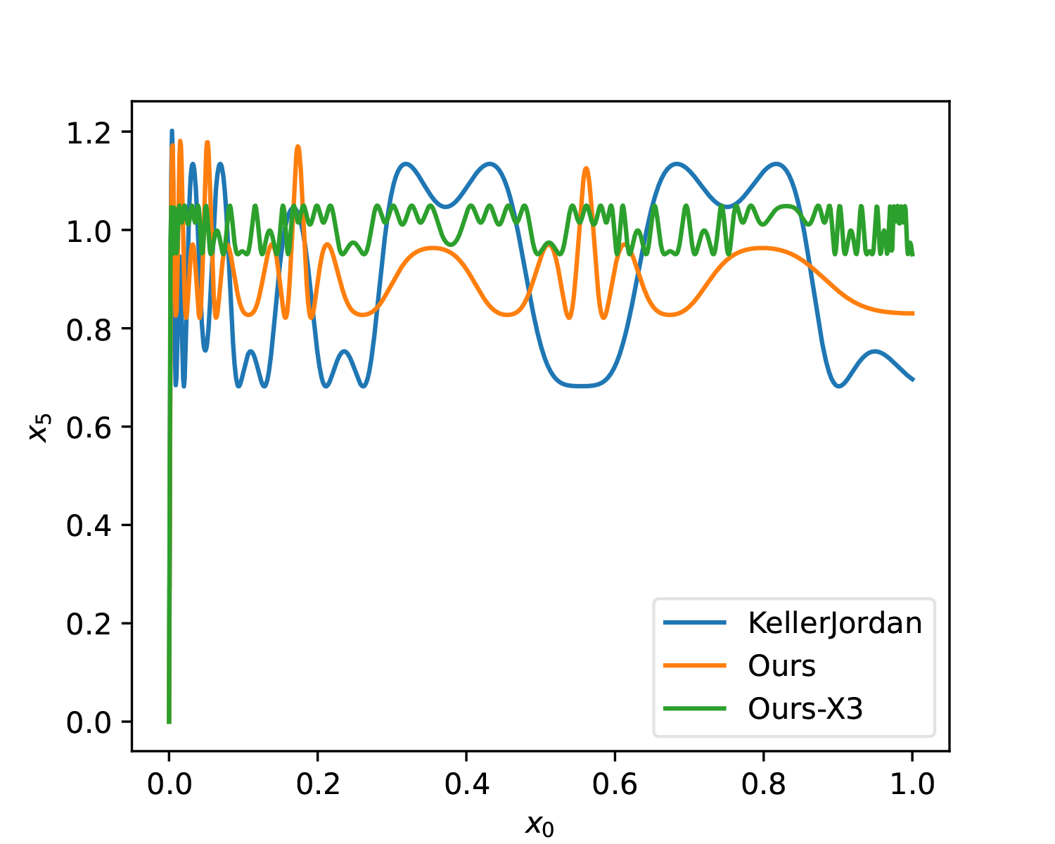
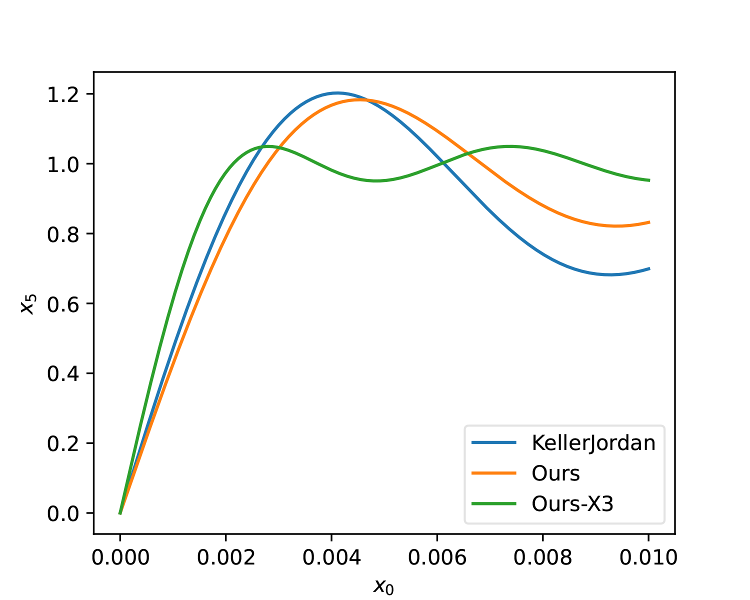
lr *= 0.1Additionally, the optimizer was changed from SGD to Adam, which makes it easier to control the update magnitude of parameters. To enhance the solution’s resistance to noise, we add some perturbation to a, b, c and mix in the gradients after perturbation. The optimization result of the above script is: (a, b, c) = (3.3748, -4.6969, 2.1433) It can be seen that this is not far from KellerJordan’s solution. Let’s further compare the differences between the two through images:
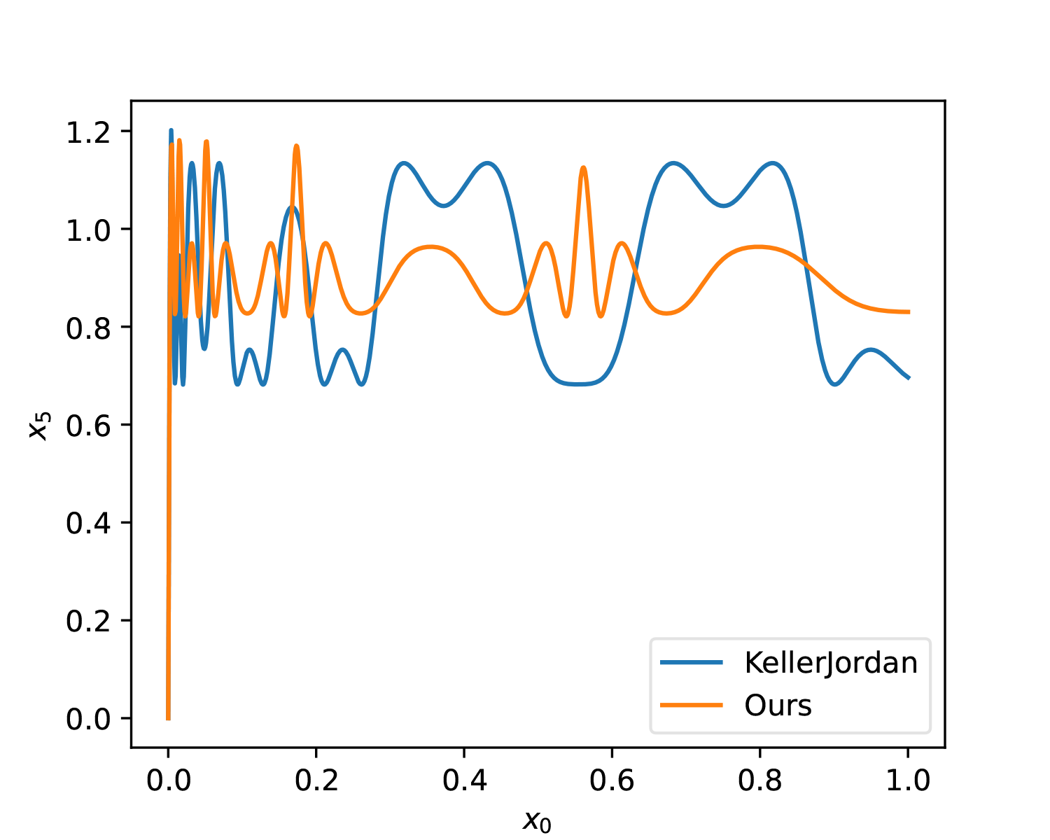
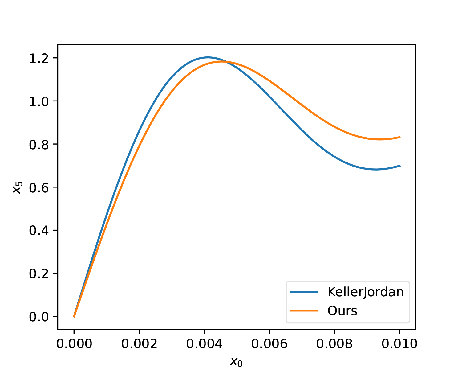
As can be seen, from a global perspective, the solution we found here has a slightly smaller average error. The advantage of KellerJordan’s solution is that the slope in the [0, 0.01] interval is slightly larger, which means it is more beneficial for smaller singular values.
Initial Value Distribution
Before further discussion, we need to clarify one question: how small are the singular values we actually care about? This goes back to the distribution of \boldsymbol{S}_0. Since \boldsymbol{S}_0 is normalized by the Frobenius norm, \mathop{\text{diag}}(\boldsymbol{S}_0) is actually an r-dimensional unit vector. If all singular values are equal, then each singular value is 1/\sqrt{r}.
Thus, according to the pigeonhole principle, in non-uniform cases, there must exist singular values smaller than 1/\sqrt{r}. To be safe, we can consider a multiple, say 10 times, which means we should at least account for singular values of size 0.1/\sqrt{r}. In practice, the probability of a matrix being strictly low-rank (i.e., singular values strictly equal to 0) is very small, so we generally assume the matrix is full-rank, i.e., r = \min(n, m). Therefore, we should at least account for 0.1/\sqrt{\min(n, m)} singular values.
Considering that for current large LLMs, the hidden_size
has reached the level of 8192 \sim
100^2, based on this estimate, a universal Muon optimizer’s \mathop{\text{msign}} algorithm should at
least account for singular values of size 0.001. That is, it should be able to map
0.001 to a value close to 1. From this
perspective, both KellerJordan’s solution and our newly found solution
are somewhat lacking.
Note: Regarding the discussion of initial value distribution, one can also refer to "Iterative Orthogonalization Scaling Laws".
Unlocking Constraints
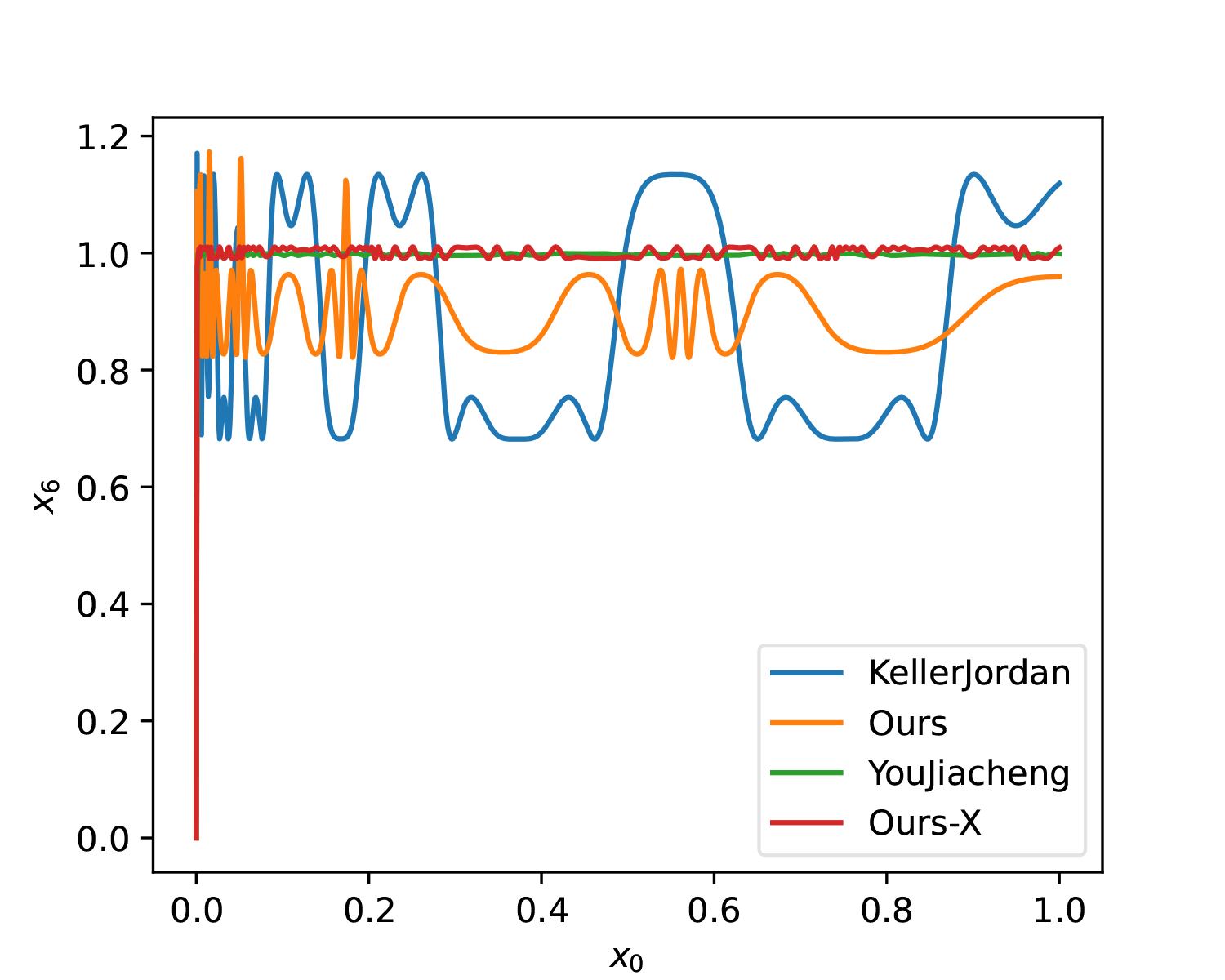
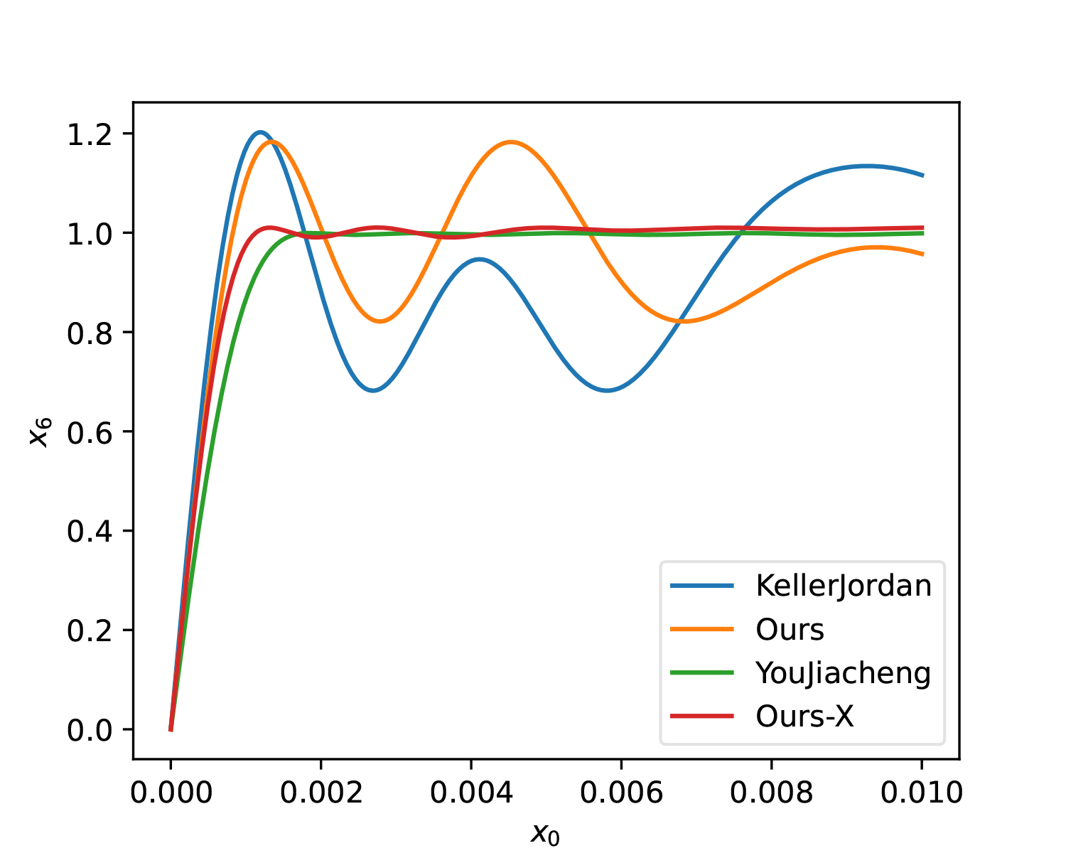
At this point, @YouJiacheng (one of the main promoters of Muon) on Twitter proposed a very clever idea: we can use different coefficients for each iteration step! That is, change the iteration to: \boldsymbol{X}_{t+1} = a_{t+1}\boldsymbol{X}_t + b_{t+1}\boldsymbol{X}_t(\boldsymbol{X}_t^{\top}\boldsymbol{X}_t) + c_{t+1}\boldsymbol{X}_t(\boldsymbol{X}_t^{\top}\boldsymbol{X}_t)^2 The benefit of this change is that once T is chosen, the total computational cost does not change at all. However, from a fitting perspective, what were originally only 3 training parameters have now become 3T, and the fitting capability will be greatly enhanced. The reference result he provided is a 6-step iteration:
| t | a | b | c |
|---|---|---|---|
| 1 | 3955/1024 | -8306/1024 | 5008/1024 |
| 2 | 3735/1024 | -6681/1024 | 3463/1024 |
| 3 | 3799/1024 | -6499/1024 | 3211/1024 |
| 4 | 4019/1024 | -6385/1024 | 2906/1024 |
| 5 | 2677/1024 | -3029/1024 | 1162/1024 |
| 6 | 2172/1024 | -1833/1024 | 682/1024 |
We can plot it for comparison:
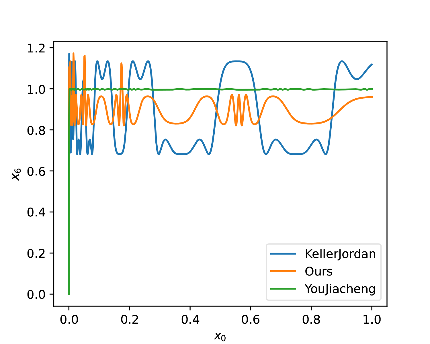
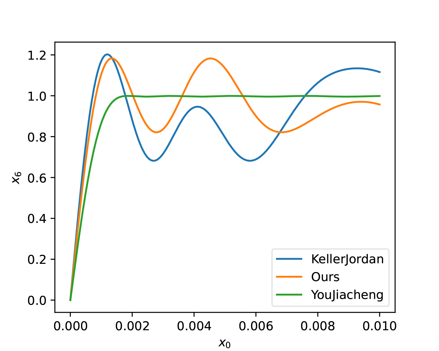
For fairness, KellerJordan’s solution and our solution were also changed to T=6. As can be seen, whether in terms of smoothness or overall approximation, YouJiacheng’s solution shows a very significant improvement, fully demonstrating the "full form" power released after removing parameter sharing.
Try it Yourself
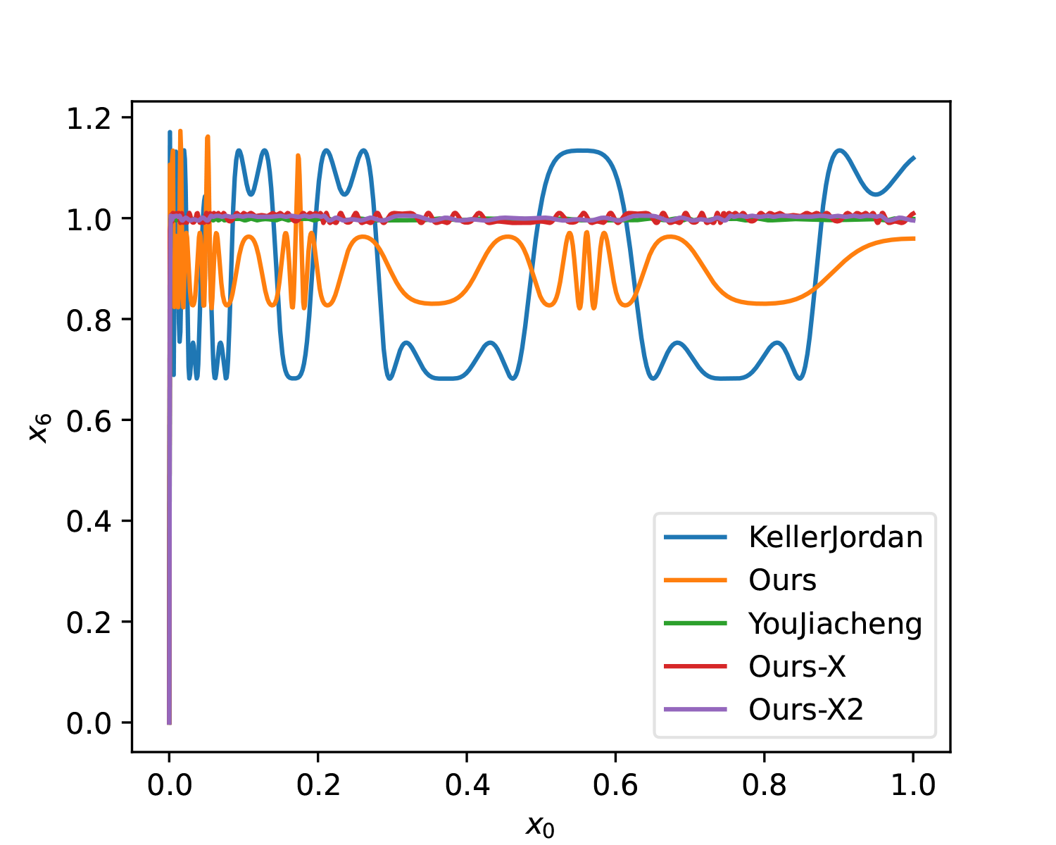
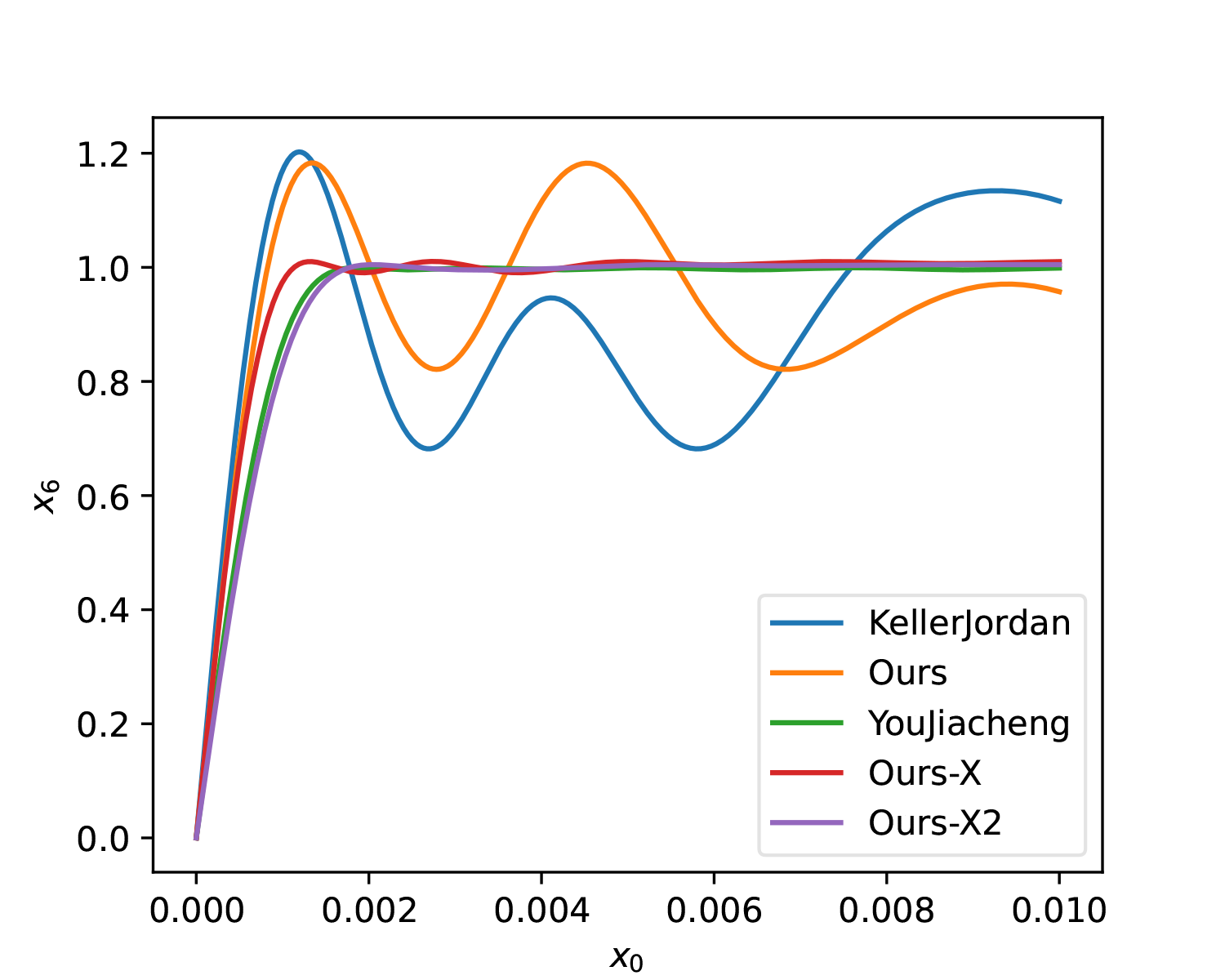
How was YouJiacheng’s solution obtained? The author shared his code here. The idea is also to use Adam for solving, but it includes many different Losses, which is a bit complicated to understand. In fact, using our previous script with the initialization he provided, we can get equally good results:
| t | a | b | c |
|---|---|---|---|
| 1 | 4140/1024 | -7553/1024 | 3571/1024 |
| 2 | 3892/1024 | -6637/1024 | 2973/1024 |
| 3 | 3668/1024 | -6456/1024 | 3021/1024 |
| 4 | 3248/1024 | -6211/1024 | 3292/1024 |
| 5 | 2792/1024 | -5759/1024 | 3796/1024 |
| 6 | 3176/1024 | -5507/1024 | 4048/1024 |
Reference code:
import jax
import jax.numpy as jnp
from tqdm import tqdm

def loss(w, x, k=50):
    for a, b, c in w:
        x = a * x + b * x**3 + c * x**5
    return jnp.abs(x - 1).sort()[-k:].mean()

@jax.jit
def grad(w, x, tol=0.1):
    G = lambda w, x: (g := jax.grad(loss)(w, x)) / jnp.fmax(jnp.linalg.norm(g), 1)
    return 0.6 * G(w, x) + 0.2 * (G(w + tol / 2, x) + G(w - tol / 2, x))

iters = 6
x = jnp.linspace(0, 1, 10001)[1:]
w = jnp.array([[3.5, -6.04444444444, 2.84444444444]] * iters)
m, v = jnp.zeros_like(w), jnp.zeros_like(w)
lr = 1e-3
pbar = tqdm(range(20000), ncols=0, desc='Adam')

for i in pbar:
    l, g = loss(w, x), grad(w, x)
    m = 0.9 * m + 0.1 * g
    v = 0.999 * v + 0.001 * g**2
    w = w - lr * m / jnp.sqrt(v + 1e-20)
    pbar.set_description(f'Loss: {l:.6f}, LR: {lr:.6f}')
    if i in [10000]:
        lr *= 0.1
Comparison below (labeled as "Ours-X"):
As seen from the figures, compared to YouJiacheng’s solution, our results oscillate more but gain a larger slope at [0, 0.001].
Other Solution Sets
If readers want a solution with fewer oscillations, they only need to increase the k value. For example, the result for k=200 is:
| t | a | b | c |
|---|---|---|---|
| 1 | 4059/1024 | -7178/1024 | 3279/1024 |
| 2 | 3809/1024 | -6501/1024 | 2925/1024 |
| 3 | 3488/1024 | -6308/1024 | 3063/1024 |
| 4 | 2924/1024 | -5982/1024 | 3514/1024 |
| 5 | 2439/1024 | -5439/1024 | 4261/1024 |
| 6 | 3148/1024 | -5464/1024 | 4095/1024 |
At this point, it is almost identical to YouJiacheng’s solution (Ours-X2):
Additionally, here is a 5-step solution for comparison with the original solution:
| t | a | b | c |
|---|---|---|---|
| 1 | 4.6182 | -12.9582 | 9.3299 |
| 2 | 3.8496 | -7.9585 | 4.3052 |
| 3 | 3.5204 | -7.2918 | 4.0606 |
| 4 | 3.2067 | -6.8243 | 4.2802 |
| 5 | 3.2978 | -5.7848 | 3.8917 |
Effect diagram (Ours-X3):
Improved Initial Values
So far, our solving for a, b, c has concluded. Overall, using different a, b, c for each step indeed significantly improves the convergence properties of Newton-Schulz iteration without adding any computational cost—it can be considered a free lunch.
Besides optimizing the coefficients of Newton-Schulz iteration, are there other ideas to improve the convergence properties? Yes, there are. @johanwind, @YouJiacheng, @ZhangRuichong, and others found that we can use the characteristics of Newton-Schulz iteration to improve the quality of initial values almost for free, thereby increasing the convergence speed. @leloykun provided a reference implementation here.
Specifically, most current efforts to improve Newton-Schulz iteration can be summarized as "maximizing the convergence speed of singular values near zero while ensuring convergence." If we can amplify these near-zero singular values beforehand, we can increase the convergence speed without changing the iteration algorithm. Currently, to compress singular values into [0, 1], we use Frobenius norm normalization \boldsymbol{M}/\Vert\boldsymbol{M}\Vert_F, which compresses singular values into: \sigma_i \quad \to \quad \frac{\sigma_i}{\Vert\boldsymbol{M}\Vert_F} = \frac{\sigma_i}{\sqrt{\sum\limits_{j=1}^r \sigma_i^2}} \in [0, 1] This does achieve the goal, but it also has the problem of over-compression. The most compact compression method should be \sigma_i \to \sigma_i/\sigma_1, i.e., spectral normalization. The problem is that the spectral norm is not as easy to calculate as the Frobenius norm, so we were forced to choose the Frobenius norm. However, we have: \sigma_1 \quad \leq \quad \underbrace{\sqrt[\uproot{10}8]{\sum_{j=1}^r \sigma_i^8}}_{\sqrt[4]{\Vert(\boldsymbol{M}^{\top}\boldsymbol{M})^2\Vert_F}} \quad \leq \quad \underbrace{\sqrt[\uproot{10}4]{\sum_{j=1}^r \sigma_i^4}}_{\sqrt{\Vert\boldsymbol{M}^{\top}\boldsymbol{M}\Vert_F}} \quad \leq \quad \underbrace{\sqrt{\sum_{j=1}^r \sigma_i^2}}_{\Vert\boldsymbol{M}\Vert_F} This means using \sqrt[4]{\Vert(\boldsymbol{M}^{\top}\boldsymbol{M})^2\Vert_F} or \sqrt{\Vert\boldsymbol{M}^{\top}\boldsymbol{M}\Vert_F} as the normalization factor is theoretically better than \Vert\boldsymbol{M}\Vert_F. Very cleverly, under Newton-Schulz iteration, their calculation is almost free! To understand this, we write the first step of iteration: \boldsymbol{X}_0 = \frac{\boldsymbol{M}}{\Vert\boldsymbol{M}\Vert_F}, \qquad \boldsymbol{X}_1 = a\boldsymbol{X}_0 + b\boldsymbol{X}_0(\boldsymbol{X}_0^{\top}\boldsymbol{X}_0) + c\boldsymbol{X}_0(\boldsymbol{X}_0^{\top}\boldsymbol{X}_0)^2 We can see that \boldsymbol{X}_0^{\top}\boldsymbol{X}_0 and (\boldsymbol{X}_0^{\top}\boldsymbol{X}_0)^2 must be calculated anyway, so we can directly use them to calculate the Frobenius norm and then re-normalize. Reference code:
def msign(x, steps=5, eps=1e-20):
    a, b, c, y = 3.4445, -4.7750, 2.0315, x.astype('bfloat16')
    y = y.mT if x.shape[0] > x.shape[1] else y
    y /= ((y**2).sum(axis=[-2, -1], keepdims=True) + eps)**0.5
    for i in range(steps):
        y4 = (y2 := y @ y.mT) @ y2
        if i == 0:
            n = ((y4**2).sum(axis=[-2, -1], keepdims=True) + eps)**0.125
            y, y2, y4 = y / n, y2 / n**2, y4 / n**4
        y = a * y + (b * y2 + c * y4) @ y
    return y.mT if x.shape[0] > x.shape[1] else y
Experimental results show that for a 100 \times 100 random Gaussian matrix, the improved minimum singular values are mostly more than twice the original, and the average singular value is also closer to 1. However, the Muon author also stated that it might bring additional instability, so it has not yet been adopted into the official code.
Summary
This article introduced the optimization ideas for calculating \mathop{\text{msign}} through Newton-Schulz iteration. The results obtained can significantly improve the convergence speed and effect of the iteration compared to Muon’s official solution.
Finally, it should be pointed out that for Muon, small-scale experimental results show that there seems to be no necessary connection between the calculation accuracy of \mathop{\text{msign}} and the final effect of the model. Improving the accuracy of \mathop{\text{msign}} in small models seems only to accelerate convergence slightly in the early stages, but the final result remains unchanged. It is currently unclear whether this conclusion holds for larger-scale models.
Reprinting: Please include the original address of this article: https://kexue.fm/archives/10922
Further details: For more details on reprinting/citation, please refer to "Scientific Space FAQ".