In the article "A First Look at MuP: Cross-Model Hyperparameter Scaling Laws", we derived MuP (Maximal Update Parametrization) based on the scale invariance of forward propagation, backward propagation, loss increments, and feature changes. For some readers, this process might still seem somewhat cumbersome, though it is already significantly simplified compared to the original paper. It is worth noting that we introduced MuP relatively completely within a single post, whereas the original MuP paper is actually the fifth in the author’s Tensor Programs series!
However, the good news is that in subsequent research, "A Spectral Condition for Feature Learning", the authors discovered a new way of understanding it (hereafter referred to as the "Spectral Condition"). This approach is more intuitive and concise than both the original MuP derivation and my own, yet it yields richer results. It can be considered a higher-order version of MuP—a representative work that is both simple and sophisticated.
Preparation
As the name suggests, the Spectral Condition is related to the spectral norm. Its starting point is a fundamental inequality of the spectral norm: \Vert\boldsymbol{x}\boldsymbol{W}\Vert_2\leq \Vert\boldsymbol{x}\Vert_2 \Vert\boldsymbol{W}\Vert_2\label{neq:spec-2} where \boldsymbol{x}\in\mathbb{R}^{d_{in}} and \boldsymbol{W}\in\mathbb{R}^{d_{in}\times d_{out}}. As for \Vert\cdot\Vert_2, we can call it the "2-norm." For \boldsymbol{x} and \boldsymbol{x}\boldsymbol{W}, which are vectors, the 2-norm is simply the vector length (Euclidean norm). For the matrix \boldsymbol{W}, its 2-norm is also known as the spectral norm, which is defined as the smallest constant C such that \Vert\boldsymbol{x}\boldsymbol{W}\Vert_2\leq C\Vert\boldsymbol{x}\Vert_2 holds for all \boldsymbol{x}. In other words, the above inequality is a direct consequence of the definition of the spectral norm and requires no additional proof.
For more on the spectral norm, readers can refer to blog posts such as "Lipschitz Constraints in Deep Learning: Generalization and Generative Models" and "The Road to Low-Rank Approximation (II): SVD". Matrices also have a simpler F-norm (Frobenius norm), which is a straightforward generalization of vector length: \Vert \boldsymbol{W}\Vert_F = \sqrt{\sum_{i=1}^{d_{in}}\sum_{j=1}^{d_{out}}W_{i,j}^2} From the perspective of singular values, the spectral norm equals the largest singular value, while the F-norm equals the square root of the sum of the squares of all singular values. Similarly, we can define the "Nuclear Norm," which is the sum of all singular values: \Vert \boldsymbol{W}\Vert_* = \sum_{i=1}^{\min(d_{in}, d_{out})} \sigma_i Matrix norms that can be expressed in terms of singular values, such as the spectral norm, F-norm, and nuclear norm, all belong to the class of Schatten-p norms. Finally, we define the RMS (Root Mean Square), which is a variant of the vector length: \Vert\boldsymbol{x}\Vert_{RMS} = \sqrt{\frac{1}{d_{in}}\sum_{i=1}^{d_{in}} x_i^2} = \frac{1}{\sqrt{d_{in}}}\Vert \boldsymbol{x}\Vert_2 If generalized to matrices, it would be \Vert\boldsymbol{W}\Vert_{RMS} = \Vert \boldsymbol{W}\Vert_F/\sqrt{d_{in} d_{out}}. The name is self-explanatory: while vector length or the matrix F-norm can be thought of as "Root Sum Square," RMS replaces the "Sum" with the "Mean." It primarily serves as an indicator of the average scale of vector or matrix elements. Substituting RMS into inequality [neq:spec-2], we obtain: \Vert\boldsymbol{x}\boldsymbol{W}\Vert_{RMS}\leq \sqrt{\frac{d_{in}}{d_{out}}}\Vert\boldsymbol{x}\Vert_{RMS} \Vert\boldsymbol{W}\Vert_2\label{neq:spec-rms}
Desired Properties
Our previous approach to deriving MuP involved a careful analysis of the forms of forward propagation, backward propagation, loss increments, and feature changes, achieving scale invariance by adjusting initialization and learning rates. The Spectral Condition, after "distilling the essence," finds that focusing on forward propagation and feature changes is sufficient.
Simply put, the Spectral Condition expects the output and the increment of every layer to be scale-invariant. If we denote each layer as \boldsymbol{x}_k= f(\boldsymbol{x}_{k-1}; \boldsymbol{W}_k), this statement translates to "expecting each \Vert\boldsymbol{x}_k\Vert_{RMS} and \Vert\Delta\boldsymbol{x}_k\Vert_{RMS} to be \Theta(1)" (where \Theta is the Big Theta Notation):
1. \Vert\boldsymbol{x}_k\Vert_{RMS}=\Theta(1) represents the stability of forward propagation, a requirement also included in the previous article’s derivation.
2. \Delta\boldsymbol{x}_k represents the change in \boldsymbol{x}_k caused by parameter updates. Thus, \Vert\Delta\boldsymbol{x}_k\Vert_{RMS}=\Theta(1) merges the requirements of backward propagation and feature changes.
We can prove that if \Vert\boldsymbol{x}_k\Vert_{RMS}=\Theta(1) and \Vert\Delta\boldsymbol{x}_k\Vert_{RMS}=\Theta(1) hold for every layer, then \Delta\mathcal{L} is automatically \Theta(1). This is the first elegant aspect of the Spectral Condition: it reduces the four conditions originally needed for MuP to just two.
The proof is not difficult. The key is our assumption that \Vert\boldsymbol{x}_k\Vert_{RMS}=\Theta(1) and \Vert\Delta\boldsymbol{x}_k\Vert_{RMS}=\Theta(1) hold for every layer, including the final layer. Suppose the model has K layers and the loss function for a single sample is \ell(\boldsymbol{x}_K). According to the assumption, \Vert\boldsymbol{x}_K\Vert_{RMS} is \Theta(1), so \ell(\boldsymbol{x}_K) is naturally \Theta(1). Since \Vert\Delta\boldsymbol{x}_K\Vert_{RMS} is \Theta(1), then \Vert\boldsymbol{x}_K + \Delta\boldsymbol{x}_K\Vert_{RMS}\leq \Vert\boldsymbol{x}_K\Vert_{RMS} + \Vert\Delta\boldsymbol{x}_K\Vert_{RMS} is also \Theta(1), making \ell(\boldsymbol{x}_K + \Delta\boldsymbol{x}_K) a \Theta(1) quantity. Thus: \Delta \ell = \ell(\boldsymbol{x}_K + \Delta\boldsymbol{x}_K) - \ell(\boldsymbol{x}_K) = \Theta(1) Therefore, the loss increment for a single sample \Delta \ell is \Theta(1). Since \Delta\mathcal{L} is the average of all \Delta \ell, it is also \Theta(1).
Spectral Condition
Next, let’s see how to satisfy these two desired properties. For a linear layer \boldsymbol{x}_k = \boldsymbol{x}_{k-1} \boldsymbol{W}_k, where \boldsymbol{W}_k\in\mathbb{R}^{d_{k-1}\times d_k}, to satisfy \Vert\boldsymbol{x}_k\Vert_{RMS}=\Theta(1), we directly apply inequality [neq:spec-rms]: \Vert\boldsymbol{x}_k\Vert_{RMS}\leq \sqrt{\frac{d_{k-1}}{d_k}}\Vert\boldsymbol{x}_{k-1}\Vert_{RMS}\, \Vert\boldsymbol{W}_k\Vert_2 If the input \Vert\boldsymbol{x}_{k-1}\Vert_{RMS} is already \Theta(1), then to ensure the output \Vert\boldsymbol{x}_k\Vert_{RMS}=\Theta(1), we need: \sqrt{\frac{d_{k-1}}{d_k}}\Vert\boldsymbol{W}_k\Vert_2 = \Theta(1)\quad\Rightarrow\quad \Vert\boldsymbol{W}_k\Vert_2 = \Theta\left(\sqrt{\frac{d_k}{d_{k-1}}}\right)\label{eq:spec-c1} This establishes the first Spectral Condition—the requirement for the spectral norm of \boldsymbol{W}_k.
After analyzing \Vert\boldsymbol{x}_k\Vert_{RMS}, we turn to \Vert\Delta\boldsymbol{x}_k\Vert_{RMS}. The increment \Delta\boldsymbol{x}_k comes from parameter changes \Delta \boldsymbol{W}_k and input changes \Delta\boldsymbol{x}_{k-1}: \begin{aligned} \Delta\boldsymbol{x}_k =&\, (\boldsymbol{x}_{k-1} + \Delta\boldsymbol{x}_{k-1})(\boldsymbol{W}_k+\Delta \boldsymbol{W}_k) - \boldsymbol{x}_{k-1}\boldsymbol{W}_k \\[5pt] =&\, \boldsymbol{x}_{k-1} (\Delta \boldsymbol{W}_k) + (\Delta\boldsymbol{x}_{k-1})\boldsymbol{W}_k + (\Delta\boldsymbol{x}_{k-1})(\Delta \boldsymbol{W}_k) \end{aligned} Applying the RMS norm: \begin{aligned} \Vert\Delta\boldsymbol{x}_k\Vert_{RMS} =&\, \Vert\boldsymbol{x}_{k-1} (\Delta \boldsymbol{W}_k) + (\Delta\boldsymbol{x}_{k-1})\boldsymbol{W}_k + (\Delta\boldsymbol{x}_{k-1})(\Delta \boldsymbol{W}_k)\Vert_{RMS} \\[5pt] \leq&\, \Vert\boldsymbol{x}_{k-1} (\Delta \boldsymbol{W}_k)\Vert_{RMS} + \Vert(\Delta\boldsymbol{x}_{k-1})\boldsymbol{W}_k\Vert_{RMS} + \Vert(\Delta\boldsymbol{x}_{k-1})(\Delta \boldsymbol{W}_k)\Vert_{RMS} \\[5pt] \leq&\, \sqrt{\frac{d_{k-1}}{d_k}}\left({\begin{gathered}\Vert\boldsymbol{x}_{k-1}\Vert_{RMS}\,\Vert\Delta \boldsymbol{W}_k\Vert_2 + \Vert\Delta\boldsymbol{x}_{k-1}\Vert_{RMS}\,\Vert \boldsymbol{W}_k\Vert_2 \\[5pt] + \Vert\Delta\boldsymbol{x}_{k-1}\Vert_{RMS}\,\Vert\Delta \boldsymbol{W}_k\Vert_2\end{gathered}} \right) \end{aligned} Analyzing term by term: \underbrace{\Vert\boldsymbol{x}_{k-1}\Vert_{RMS}}_{\Theta(1)}\,\Vert\Delta \boldsymbol{W}_k\Vert_2 + \underbrace{\Vert\Delta\boldsymbol{x}_{k-1}\Vert_{RMS}}_{\Theta(1)}\,\underbrace{\Vert \boldsymbol{W}_k\Vert_2}_{\Theta\left(\sqrt{\frac{d_k}{d_{k-1}}}\right)} + \underbrace{\Vert\Delta\boldsymbol{x}_{k-1}\Vert_{RMS}}_{\Theta(1)}\,\Vert\Delta \boldsymbol{W}_k\Vert_2 To ensure \Vert\Delta\boldsymbol{x}_k\Vert_{RMS}=\Theta(1), we need: \Vert\Delta\boldsymbol{W}_k\Vert_2 = \Theta\left(\sqrt{\frac{d_k}{d_{k-1}}}\right)\label{eq:spec-c2} This is the second Spectral Condition—the requirement for the spectral norm of \Delta\boldsymbol{W}_k.
Spectral Normalization
Now that we have the two spectral conditions [eq:spec-c1] and [eq:spec-c2], we need to design the model and optimization to satisfy them.
The standard way to make a matrix satisfy a spectral norm condition is Spectral Normalization (SN). First, for initialization, we can take any random matrix \boldsymbol{W}_k' and normalize it: \boldsymbol{W}_k = \sigma\sqrt{\frac{d_k}{d_{k-1}}}\frac{\boldsymbol{W}_k'}{\Vert\boldsymbol{W}_k'\Vert_2} where \sigma > 0 is a scale-invariant constant. Similarly, for any update \boldsymbol{\Phi}_k provided by an optimizer, we can construct \Delta \boldsymbol{W}_k via spectral normalization: \Delta \boldsymbol{W}_k = \eta\sqrt{\frac{d_k}{d_{k-1}}}\frac{\boldsymbol{\Phi}_k}{\Vert\boldsymbol{\Phi}_k\Vert_2} where \eta > 0 is the learning rate. This ensures \Vert\Delta\boldsymbol{W}_k\Vert_2=\Theta\left(\sqrt{\frac{d_k}{d_{k-1}}}\right) at every step.
Singular Value Clipping
Besides Spectral Normalization, we can consider Singular Value Clipping (SVC). This part is my own addition and does not appear in the original paper, but it explains some interesting results.
SVC clips singular values that are greater than 1 to 1, while leaving those less than or equal to 1 unchanged: \mathop{\text{SVC}}(\boldsymbol{W}) = \boldsymbol{U}\min(\boldsymbol{\Lambda},1)\boldsymbol{V}^{\top},\qquad \boldsymbol{U},\boldsymbol{\Lambda},\boldsymbol{V}^{\top} = \text{SVD}(\boldsymbol{W}) In contrast, SN is \text{SN}(\boldsymbol{W})=\boldsymbol{U}(\boldsymbol{\Lambda}/\max(\boldsymbol{\Lambda}))\boldsymbol{V}^{\top}. Using SVC: \boldsymbol{W}_k = \sigma\sqrt{\frac{d_k}{d_{k-1}}}\mathop{\text{SVC}}(\boldsymbol{W}_k'), \qquad \Delta \boldsymbol{W}_k = \eta\sqrt{\frac{d_k}{d_{k-1}}}\mathop{\text{SVC}}(\boldsymbol{\Phi}_k) A limit version of SVC (by scaling the input by \lambda \to \infty) is the matrix sign function \mathop{\text{msign}}(\boldsymbol{W}), used in the Muon optimizer: \Delta \boldsymbol{W}_k = \eta\sqrt{\frac{d_k}{d_{k-1}}}\mathop{\text{msign}}(\boldsymbol{\Phi}_k) This gives us a generalized Muon optimizer. Recently, experiments on "Mudamw" (applying \mathop{\text{msign}} to Adam updates) showed results even better than Muon:
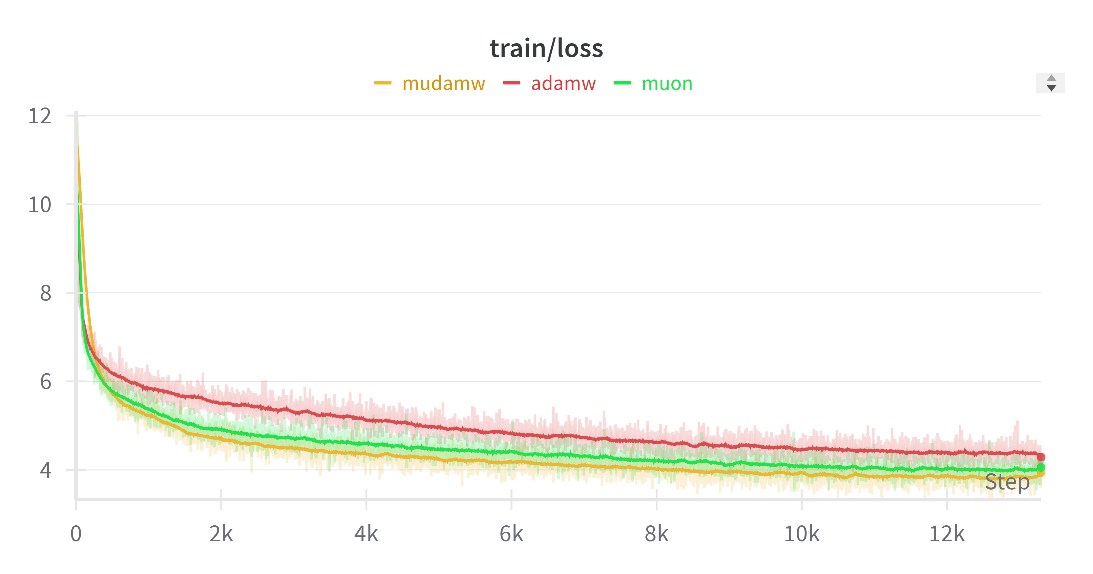
We also tried this on small models and replicated similar conclusions. This suggests that applying \mathop{\text{msign}} to existing optimizers might yield better results, which can be understood here as a limit version of singular value clipping.
Approximate Estimation
Since SVD-related operations are expensive, we seek simpler forms for scaling laws. For initialization, a d_{k-1}\times d_k matrix sampled from a standard normal distribution has a maximum singular value roughly equal to \sqrt{d_{k-1}} + \sqrt{d_k}. Thus, setting the sampling standard deviation to: \sigma_k = \Theta\left(\sqrt{\frac{d_k}{d_{k-1}}}(\sqrt{d_{k-1}} + \sqrt{d_k})^{-1}\right) = \Theta\left(\sqrt{\frac{1}{d_{k-1}}\min\left(1, \frac{d_k}{d_{k-1}}\right)}\right) \label{eq:spec-std} satisfies the initialization spectral condition.
For updates, we utilize the empirical observation that gradient matrices are often low-rank (the basis for LoRA). Under this assumption, the spectral norm and nuclear norm are of the same order: \Theta(\Vert\nabla_{\boldsymbol{W}_k}\mathcal{L}\Vert_2)=\Theta(\Vert\nabla_{\boldsymbol{W}_k}\mathcal{L}\Vert_*). Using the relationship \Delta\mathcal{L} \approx \sum_k \langle \Delta\boldsymbol{W}_k, \nabla_{\boldsymbol{W}_k}\mathcal{L}\rangle_F \leq \sum_k \Vert\Delta\boldsymbol{W}_k\Vert_2\, \Vert\nabla_{\boldsymbol{W}_k}\mathcal{L}\Vert_*, we find that when \Vert\Delta\boldsymbol{W}_k\Vert_2=\Theta\left(\sqrt{\frac{d_k}{d_{k-1}}}\right), we have: \Theta(\Vert\nabla_{\boldsymbol{W}_k}\mathcal{L}\Vert_2) = \Theta\left(\sqrt{\frac{d_{k-1}}{d_k}}\right)\label{eq:grad-norm}
Learning Rate Strategy
Applying estimate [eq:grad-norm] to SGD (\Delta \boldsymbol{W}_k = -\eta_k \nabla_{\boldsymbol{W}_k}\mathcal{L}), to achieve \Vert\Delta\boldsymbol{W}_k\Vert_2=\Theta\left(\sqrt{\frac{d_k}{d_{k-1}}}\right), we need: \eta_k = \Theta\left(\frac{d_k}{d_{k-1}}\right)\label{eq:sgd-eta}
For Adam, approximating with SignSGD (\Delta \boldsymbol{W}_k = -\eta_k \mathop{\text{sign}}(\nabla_{\boldsymbol{W}_k}\mathcal{L})), since \Vert\mathop{\text{sign}}(\nabla_{\boldsymbol{W}_k}\mathcal{L})\Vert_F = \Theta(\sqrt{d_{k-1} d_k}) and assuming low-rankness, we have \Vert\mathop{\text{sign}}(\nabla_{\boldsymbol{W}_k}\mathcal{L})\Vert_2 = \Theta(\sqrt{d_{k-1} d_k}). Thus, we need: \eta_k = \Theta\left(\frac{1}{d_{k-1}}\right)\label{eq:adam-eta}
Comparing with MuP, which treats input, hidden, and output layers separately, the Spectral Condition provides a single unified formula that covers all cases as d \to \infty. For example, for a hidden layer where d_{k-1}=d_k=d, the Adam learning rate becomes \Theta(1/d), matching MuP.
Summary
The Spectral Condition is a higher-order version of MuP that uses spectral norm inequalities to derive stable training conditions more elegantly.
\left\{ \begin{aligned} &\text{Desired Properties:} \begin{cases} \Vert\boldsymbol{x}_k\Vert_{RMS}=\Theta(1) \\ \Vert\Delta\boldsymbol{x}_k\Vert_{RMS}=\Theta(1) \end{cases} \\[10pt] &\text{Spectral Conditions:} \begin{cases} \Vert\boldsymbol{W}_k\Vert_2 = \Theta\left(\sqrt{\frac{d_k}{d_{k-1}}}\right) \\ \Vert\Delta\boldsymbol{W}_k\Vert_2 = \Theta\left(\sqrt{\frac{d_k}{d_{k-1}}}\right) \end{cases} \\[10pt] &\text{Implementation:} \\ &\quad \text{Spectral Norm:} \begin{cases} \boldsymbol{W}_k = \sigma\sqrt{\frac{d_k}{d_{k-1}}}\frac{\boldsymbol{W}_k'}{\Vert\boldsymbol{W}_k'\Vert_2} \\ \Delta \boldsymbol{W}_k = \eta\sqrt{\frac{d_k}{d_{k-1}}}\frac{\boldsymbol{\Phi}_k}{\Vert\boldsymbol{\Phi}_k\Vert_2} \end{cases} \\[10pt] &\quad \text{SVC/msign:} \begin{cases} \boldsymbol{W}_k = \sigma\sqrt{\frac{d_k}{d_{k-1}}}\mathop{\text{SVC}}(\boldsymbol{W}_k') \to \text{msign} \\ \Delta \boldsymbol{W}_k = \eta\sqrt{\frac{d_k}{d_{k-1}}}\mathop{\text{SVC}}(\boldsymbol{\Phi}_k) \to \text{msign} \end{cases} \\[10pt] &\text{Approx. Estimation:} \begin{cases} \sigma_k = \Theta\left(\sqrt{\frac{1}{d_{k-1}}\min\left(1, \frac{d_k}{d_{k-1}}\right)}\right) \\ \eta_k = \begin{cases} \text{SGD: } \Theta\left(\frac{d_k}{d_{k-1}}\right) \\ \text{Adam: } \Theta\left(\frac{1}{d_{k-1}}\right) \end{cases} \end{cases} \end{aligned} \right.
Original Address: https://kexue.fm/archives/10795