A few days ago, I came across a new paper on arXiv titled "Compressed Image Generation with Denoising Diffusion Codebook Models". I was truly impressed by the author’s bold creativity and couldn’t help but share it with everyone.
As the title suggests, the author proposes a creative idea called DDCM (Denoising Diffusion Codebook Models). It restricts the noise sampling of DDPM to a finite set, which enables some wonderful effects, such as encoding samples into discrete ID sequences and reconstructing them, much like VQVAE. Note that these operations are performed on a pre-trained DDPM without any additional training.
Finite Sets
Since DDCM only requires a pre-trained DDPM model to perform sampling, we will not repeat the model details of DDPM here. Readers who are not yet familiar with DDPM can review parts (1), (2), and (3) of our "Generative Diffusion Models" series.
We know that DDPM generation sampling starts from \boldsymbol{x}_T \sim \mathcal{N}(\boldsymbol{0}, \boldsymbol{I}) and iterates to \boldsymbol{x}_0 using the following formula: \boldsymbol{x}_{t-1} = \boldsymbol{\mu}(\boldsymbol{x}_t) + \sigma_t \boldsymbol{\varepsilon}_t,\quad \boldsymbol{\varepsilon}_t \sim \mathcal{N}(\boldsymbol{0}, \boldsymbol{I})\label{eq:ddpm-g} For DDPM, a noise vector needs to be sampled at each iteration step. Since \boldsymbol{x}_T itself is also sampled noise, a total of T+1 noise vectors are passed in during the process of generating \boldsymbol{x}_0 through T iterations. Assuming \boldsymbol{x}_t \in \mathbb{R}^d, the DDPM sampling process is actually a mapping from \mathbb{R}^{d \times (T+1)} \mapsto \mathbb{R}^d.
The first brilliant idea of DDCM is to change the noise sampling space to a finite set (Codebook): \boldsymbol{x}_{t-1} = \boldsymbol{\mu}(\boldsymbol{x}_t) + \sigma_t \boldsymbol{\varepsilon}_t,\quad \boldsymbol{\varepsilon}_t \sim \mathcal{C}_t\label{eq:ddcm-g} and \boldsymbol{x}_T \sim \mathcal{C}_{T+1}, where \mathcal{C}_t is a set of K noise vectors pre-sampled from \mathcal{N}(\boldsymbol{0}, \boldsymbol{I}). In other words, before sampling, K vectors are sampled from \mathcal{N}(\boldsymbol{0}, \boldsymbol{I}) and fixed. Every subsequent sampling step uniformly picks from these K vectors. Consequently, the generation process becomes a mapping from \{1, 2, \dots, K\}^{T+1} \mapsto \mathbb{R}^d.
What is the loss in generation quality for doing this? DDCM conducted experiments and found the loss to be very small:
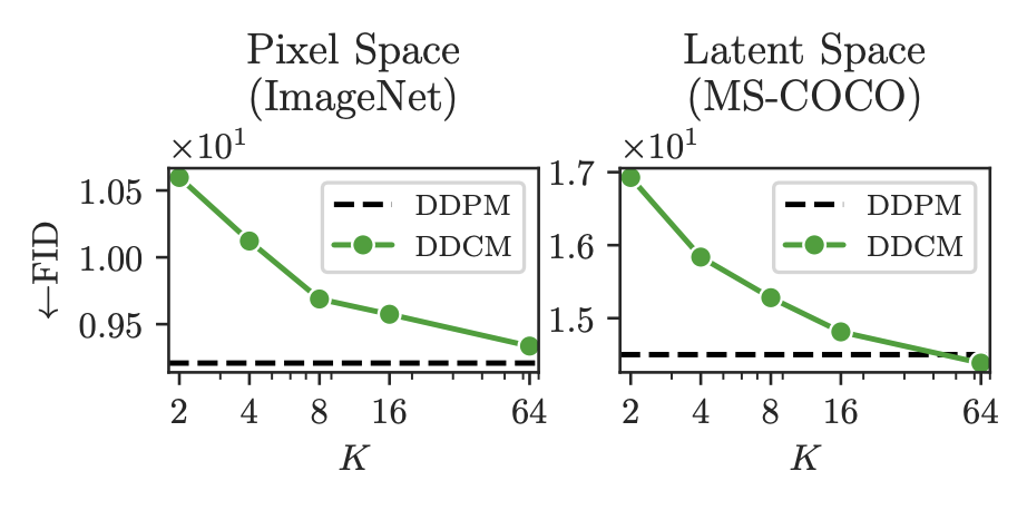
As can be seen, when K = 64, the FID basically catches up with the original. Upon closer observation, one finds that even at K=2, not much is lost. This indicates that limiting the sampling space can maintain the generative capability of DDPM. Note a detail here: \mathcal{C}_t at each step is independent, meaning there are (T+1)K total noises across all codebooks, rather than sharing K noises. I performed a simple reproduction and found that if they are shared, K \geq 8192 is required to maintain similar performance.
Discrete Encoding
Now let us consider an inverse problem: finding the discrete encoding for a given \boldsymbol{x}_0, i.e., finding the corresponding sequence \boldsymbol{\varepsilon}_T \in \mathcal{C}_T, \dots, \boldsymbol{\varepsilon}_1 \in \mathcal{C}_1 such that the \boldsymbol{x}_0 generated by the iteration \boldsymbol{x}_{t-1} = \boldsymbol{\mu}(\boldsymbol{x}_t) + \sigma_t \boldsymbol{\varepsilon}_t is as close as possible to the given sample.
Since the FID does not change significantly after limiting the sampling space, we can assume that all samples from the same distribution can be generated via Equation [eq:ddcm-g]. Therefore, a solution to the above inverse problem theoretically exists. But how do we find it? An intuitive idea is to work backward from \boldsymbol{x}_0, but upon reflection, this is difficult to operate. For example, in the first step \boldsymbol{x}_0 = \boldsymbol{\mu}(\boldsymbol{x}_1) + \sigma_1 \boldsymbol{\varepsilon}_1, both \boldsymbol{x}_1 and \boldsymbol{\varepsilon}_1 are unknown, making it hard to determine both simultaneously.
This is where DDCM’s second brilliant idea comes in: it treats the discrete encoding of \boldsymbol{x}_0 as a conditional control generation problem! Specifically, starting from a fixed \boldsymbol{x}_T, we select \boldsymbol{\varepsilon}_t in the following way: \boldsymbol{x}_{t-1} = \boldsymbol{\mu}(\boldsymbol{x}_t) + \sigma_t \boldsymbol{\varepsilon}_t,\quad \boldsymbol{\varepsilon}_t = \mathop{\text{argmax}}_{\boldsymbol{\varepsilon}\in\mathcal{C}_t} \boldsymbol{\varepsilon}\cdot(\boldsymbol{x}_0-\bar{\boldsymbol{\mu}}(\boldsymbol{x}_t))\label{eq:ddcm-eg} Here \bar{\boldsymbol{\mu}}(\boldsymbol{x}_t) is the model that predicts \boldsymbol{x}_0 using \boldsymbol{x}_t. Its relationship with \boldsymbol{\mu}(\boldsymbol{x}_t) is: \boldsymbol{\mu}(\boldsymbol{x}_t) = \frac{\alpha_t\bar{\beta}_{t-1}^2}{\bar{\beta}_t^2}\boldsymbol{x}_t + \frac{\bar{\alpha}_{t-1}\beta_t^2}{\bar{\beta}_t^2}\bar{\boldsymbol{\mu}}(\boldsymbol{x}_t) If readers have forgotten this part, they can review "Generative Diffusion Models Part 3: DDPM = Bayesian + Denoising".
We will discuss the detailed derivation in the next section. For now, let’s observe Equation [eq:ddcm-eg]. The only difference from the random generation in Equation [eq:ddcm-g] is the use of \text{argmax} to select the optimal \boldsymbol{\varepsilon}_t. The metric is the inner product similarity between \boldsymbol{\varepsilon} and the residual \boldsymbol{x}_0 - \bar{\boldsymbol{\mu}}(\boldsymbol{x}_t). Intuitively, this makes \boldsymbol{\varepsilon} compensate as much as possible for the gap between the current \bar{\boldsymbol{\mu}}(\boldsymbol{x}_t) and the target \boldsymbol{x}_0. Through the iteration of Equation [eq:ddcm-eg], the image is equivalently converted into T-1 integers (\sigma_1 is usually set to zero).
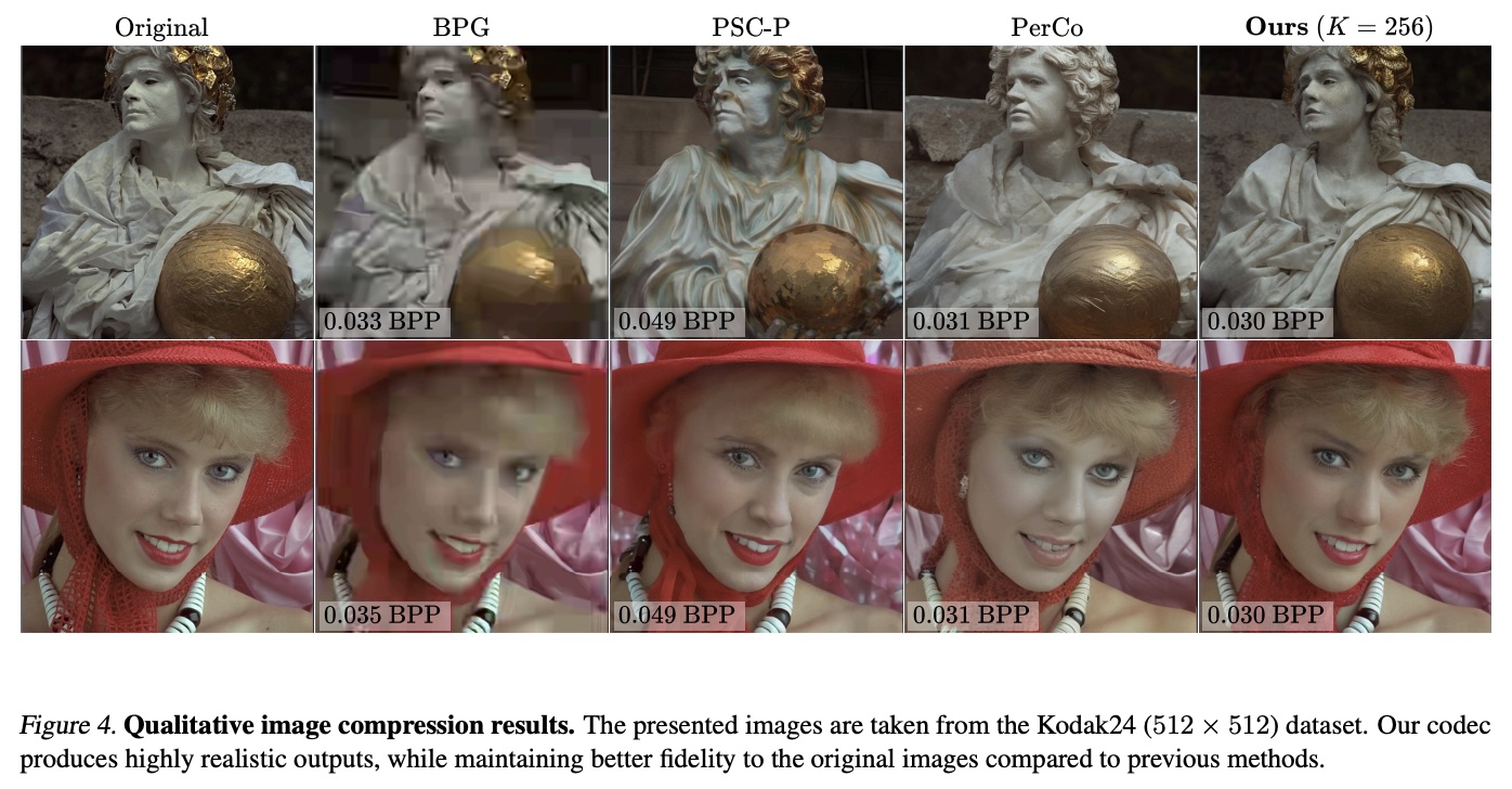
The rule looks simple, but how is the actual reconstruction effect? Below is a figure taken from the original paper. As you can see, it is quite stunning. The original paper contains even more result images. I also tried it on my own model and found that it can basically reproduce similar effects, so the method is quite reliable.
Conditional Generation
As mentioned, DDCM treats the encoding process as a conditional control generation process. How should we understand this? Starting from DDPM’s Equation [eq:ddpm-g], it can be equivalently written as: p(\boldsymbol{x}_{t-1}|\boldsymbol{x}_t) = \mathcal{N}(\boldsymbol{x}_{t-1};\boldsymbol{\mu}(\boldsymbol{x}_t),\sigma_t^2\boldsymbol{I}) Now, what we want to do is regulate the generation process given \boldsymbol{x}_0, so we add an extra condition \boldsymbol{x}_0 to the above distribution, changing it to p(\boldsymbol{x}_{t-1}|\boldsymbol{x}_t,\boldsymbol{x}_0). In fact, in DDPM, p(\boldsymbol{x}_{t-1}|\boldsymbol{x}_t,\boldsymbol{x}_0) has an analytical solution, which we derived in "Generative Diffusion Models Part 3": p(\boldsymbol{x}_{t-1}|\boldsymbol{x}_t, \boldsymbol{x}_0) = \mathcal{N}\left(\boldsymbol{x}_{t-1};\frac{\alpha_t\bar{\beta}_{t-1}^2}{\bar{\beta}_t^2}\boldsymbol{x}_t + \frac{\bar{\alpha}_{t-1}\beta_t^2}{\bar{\beta}_t^2}\boldsymbol{x}_0,\frac{\bar{\beta}_{t-1}^2\beta_t^2}{\bar{\beta}_t^2} \boldsymbol{I}\right) Or written as: \begin{aligned} \boldsymbol{x}_{t-1} =&\, \frac{\alpha_t\bar{\beta}_{t-1}^2}{\bar{\beta}_t^2}\boldsymbol{x}_t + \frac{\bar{\alpha}_{t-1}\beta_t^2}{\bar{\beta}_t^2}\boldsymbol{x}_0 + \frac{\bar{\beta}_{t-1}\beta_t}{\bar{\beta}_t}\boldsymbol{\varepsilon}_t \\ =&\, \underbrace{\frac{\alpha_t\bar{\beta}_{t-1}^2}{\bar{\beta}_t^2}\boldsymbol{x}_t + \frac{\bar{\alpha}_{t-1}\beta_t^2}{\bar{\beta}_t^2}\bar{\boldsymbol{\mu}}(\boldsymbol{x}_t)}_{\boldsymbol{\mu}(\boldsymbol{x}_t)} + \frac{\bar{\alpha}_{t-1}\beta_t^2}{\bar{\beta}_t^2}(\boldsymbol{x}_0 - \bar{\boldsymbol{\mu}}(\boldsymbol{x}_t)) + \underbrace{\frac{\bar{\beta}_{t-1}\beta_t}{\bar{\beta}_t}}_{\sigma_t}\boldsymbol{\varepsilon}_t \end{aligned}\label{eq:ddcm-eg0} where \boldsymbol{\varepsilon}_t \sim \mathcal{N}(\boldsymbol{0}, \boldsymbol{I}). Compared to Equation [eq:ddpm-g], the above equation has an additional term \boldsymbol{x}_0 - \bar{\boldsymbol{\mu}}(\boldsymbol{x}_t), which is used to guide the generation result toward \boldsymbol{x}_0. But remember our task is to discretely encode \boldsymbol{x}_0, so \boldsymbol{x}_0 cannot explicitly participate in the generation process; otherwise, it would be circular reasoning. To this end, we hope that the term \boldsymbol{x}_0 - \bar{\boldsymbol{\mu}}(\boldsymbol{x}_t) can be compensated for by \boldsymbol{\varepsilon}_t, so we adjust the selection rule for \boldsymbol{\varepsilon}_t to: \boldsymbol{\varepsilon}_t = \mathop{\text{argmin}}_{\boldsymbol{\varepsilon}\in\mathcal{C}_t} \left\Vert\frac{\bar{\alpha}_{t-1}\beta_t^2}{\bar{\beta}_t^2}(\boldsymbol{x}_0 - \bar{\boldsymbol{\mu}}(\boldsymbol{x}_t)) - \frac{\bar{\beta}_{t-1}\beta_t}{\bar{\beta}_t}\boldsymbol{\varepsilon}\right\Vert\label{eq:ddcm-eps0} Since the vectors in \mathcal{C}_t are pre-sampled from \mathcal{N}(\boldsymbol{0}, \boldsymbol{I}), similar to the "Unit Norm Lemma" in "The Amazing Johnson-Lindenstrauss Lemma: Theory", we can assume that the lengths of vectors in \mathcal{C}_t are roughly the same. Under this assumption, the above equation is equivalent to: \boldsymbol{\varepsilon}_t = \mathop{\text{argmax}}_{\boldsymbol{\varepsilon}\in\mathcal{C}_t} \boldsymbol{\varepsilon}\cdot(\boldsymbol{x}_0-\bar{\boldsymbol{\mu}}(\boldsymbol{x}_t)) This yields DDCM’s Equation [eq:ddcm-eg].
Importance Sampling
In the derivation above, we used the phrasing "hoping that the term \boldsymbol{x}_0 - \bar{\boldsymbol{\mu}}(\boldsymbol{x}_t) can be compensated for by \boldsymbol{\varepsilon}_t, so we change the selection rule to Equation [eq:ddcm-eps0]." While this seems intuitive, it is mathematically imprecise, or even strictly speaking, incorrect. In this section, we will formalize this part.
Reviewing Equation [eq:ddcm-eg0] again, the derivation up to that point is rigorous. The imprecise part lies in the way Equation [eq:ddcm-eg0] is linked to \mathcal{C}_t. Imagine what happens when K \to \infty if we select \boldsymbol{\varepsilon}_t according to [eq:ddcm-eps0]? At this point, we can consider \mathcal{C}_t to have covered the entire \mathbb{R}^d, so \frac{\bar{\alpha}_{t-1}\beta_t^2}{\bar{\beta}_t^2}(\boldsymbol{x}_0 - \bar{\boldsymbol{\mu}}(\boldsymbol{x}_t)) = \frac{\bar{\beta}_{t-1}\beta_t}{\bar{\beta}_t}\boldsymbol{\varepsilon}_t. This means Equation [eq:ddcm-eg0] becomes a deterministic transformation: \boldsymbol{x}_{t-1} = \frac{\alpha_t\bar{\beta}_{t-1}^2}{\bar{\beta}_t^2}\boldsymbol{x}_t + \frac{\bar{\alpha}_{t-1}\beta_t^2}{\bar{\beta}_t^2}\bar{\boldsymbol{\mu}}(\boldsymbol{x}_t) + \frac{\bar{\alpha}_{t-1}\beta_t^2}{\bar{\beta}_t^2}(\boldsymbol{x}_0 - \bar{\boldsymbol{\mu}}(\boldsymbol{x}_t)) = \frac{\alpha_t\bar{\beta}_{t-1}^2}{\bar{\beta}_t^2}\boldsymbol{x}_t + \frac{\bar{\alpha}_{t-1}\beta_t^2}{\bar{\beta}_t^2}\boldsymbol{x}_0 In other words, when K \to \infty, the original random sampling trajectory cannot be recovered. This is not scientifically sound. We believe that limiting the sampling space should be an approximation of the continuous sampling space; when K \to \infty, it should revert to the continuous sampling trajectory so that each step of discretization has a theoretical guarantee. Or, in a more mathematical expression, we believe a necessary condition is: \lim_{K\to\infty} \text{DDCM} = \text{DDPM}
From Equation [eq:ddpm-g] to Equation [eq:ddcm-eg0], we can also view it as the noise distribution changing from \mathcal{N}(\boldsymbol{0}, \boldsymbol{I}) to \mathcal{N}(\frac{\bar{\alpha}_{t-1}\beta_t^2}{\bar{\beta}_t^2\sigma_t}(\boldsymbol{x}_0 - \bar{\boldsymbol{\mu}}(\boldsymbol{x}_t)), \boldsymbol{I}). However, due to the encoding requirement, we cannot sample directly from the latter but only from the finite set \mathcal{C}_t. To satisfy the necessary condition—that is, to make the sampling result closer to sampling from \mathcal{N}(\frac{\bar{\alpha}_{t-1}\beta_t^2}{\bar{\beta}_t^2\sigma_t}(\boldsymbol{x}_0 - \bar{\boldsymbol{\mu}}(\boldsymbol{x}_t)), \boldsymbol{I})—we can weight \boldsymbol{\varepsilon} \in \mathcal{C}_t using its probability density function: p(\boldsymbol{\varepsilon})\propto \exp\left(-\frac{1}{2}\left\Vert\boldsymbol{\varepsilon} - \frac{\bar{\alpha}_{t-1}\beta_t^2}{\bar{\beta}_t^2\sigma_t}(\boldsymbol{x}_0 - \bar{\boldsymbol{\mu}}(\boldsymbol{x}_t))\right\Vert^2\right),\quad \boldsymbol{\varepsilon}\in\mathcal{C}_t\label{eq:ddcm-p} That is to say, the most reasonable way should be to perform importance sampling according to the probabilities after applying Softmax to -\frac{1}{2}\left\Vert\boldsymbol{\varepsilon} - \frac{\bar{\alpha}_{t-1}\beta_t^2}{\bar{\beta}_t^2\sigma_t}(\boldsymbol{x}_0 - \bar{\boldsymbol{\mu}}(\boldsymbol{x}_t))\right\Vert^2, rather than directly taking the \text{argmax}. It’s just that when K is small, the distribution after Softmax will be close to a one-hot distribution, so sampling by probability is approximately equal to \text{argmax}.
General Form
We can also extend the above results to Classifier-Guidance generation. According to the derivation in "Generative Diffusion Models Part 9: Conditional Control Results", the result of adding Classifier-Guidance to Equation [eq:ddpm-g] is: \boldsymbol{x}_{t-1} = \boldsymbol{\mu}(\boldsymbol{x}_t) + \sigma_t^2 \nabla_{\boldsymbol{x}_t} \log p(\boldsymbol{y}|\boldsymbol{x}_t) + \sigma_t\boldsymbol{\varepsilon}_t,\quad \boldsymbol{\varepsilon}_t\sim \mathcal{N}(\boldsymbol{0},\boldsymbol{I}) That is, \sigma_t^2 \nabla_{\boldsymbol{x}_t} \log p(\boldsymbol{y}|\boldsymbol{x}_t) is added, where p(\boldsymbol{y}|\boldsymbol{x}_t) is a noisy sample classifier. If we only have a clean sample classifier p_o(\boldsymbol{y}|\boldsymbol{x}), we can let p(\boldsymbol{y}|\boldsymbol{x}_t) = p_{o}(\boldsymbol{y}|\boldsymbol{\mu}(\boldsymbol{x}_t)).
Under the same derivation, we can obtain a selection rule similar to Equation [eq:ddcm-eps0]: \boldsymbol{\varepsilon}_t = \mathop{\text{argmin}}_{\boldsymbol{\varepsilon}\in\mathcal{C}_t} \left\Vert\sigma_t^2 \nabla_{\boldsymbol{x}_t} \log p(\boldsymbol{y}|\boldsymbol{x}_t) - \sigma_t\boldsymbol{\varepsilon}\right\Vert Or approximately: \boldsymbol{\varepsilon}_t = \mathop{\text{argmax}}_{\boldsymbol{\varepsilon}\in\mathcal{C}_t} \boldsymbol{\varepsilon}\cdot\nabla_{\boldsymbol{x}_t} \log p(\boldsymbol{y}|\boldsymbol{x}_t) Of course, one can also construct a sampling distribution according to Equation [eq:ddcm-p]: p(\boldsymbol{\varepsilon})\propto \exp\left(-\frac{1}{2}\left\Vert\boldsymbol{\varepsilon} - \sigma_t\nabla_{\boldsymbol{x}_t} \log p(\boldsymbol{y}|\boldsymbol{x}_t)\right\Vert^2\right),\quad \boldsymbol{\varepsilon}\in\mathcal{C}_t These are just simple extensions of the previous results.
Personal Commentary
At this point, our introduction to DDCM is basically complete. For more details, please refer to the original paper. The author has not yet open-sourced the code, so I provide my own reference implementation here:
DDCM: https://github.com/bojone/Keras-DDPM/blob/main/ddcm.py
If you already have some understanding of diffusion models and have a ready-made diffusion model at hand, I strongly recommend trying it yourself. In fact, the principle of DDCM is easy to understand and the code is not difficult to write, but only by trying it yourself can you experience that stunning feeling that makes you want to applaud. The last time I had the same feeling was with the training-free large image generation technique "Upsample Guidance" introduced in "Generative Diffusion Models Part 23: SNR and Large Image Generation (Part 2)", which also reflected the author’s ingenious conception.
However, in terms of long-term influence, I personally believe Upsample Guidance is not as significant as DDCM. Because discrete encoding of images is one of the mainstream routes for multimodal LLMs, acting as an "Image Tokenizer," which is a crucial link. DDCM can be said to have opened up a brand new route outside of VQ and FSQ. Therefore, it may have more profound potential impact. In the original paper, DDCM only defined itself as a compression method, which is perhaps "underestimating itself."
As a discrete encoding model, DDCM has another very prominent advantage: its discrete encoding is naturally 1D, unlike VQ, FSQ, and other schemes where the encoding results usually retain the 2D characteristics of the image (except for models like TiTok that use Q-Former ideas to convert to 1D). This means that when using these encodings for autoregressive generation, we no longer need to consider the "ordering" problem (refer to "Discussion on Multimodal Ideas (2): Autoregression"), which makes things much simpler.
Of course, there is still room for improvement. For example, currently, encoding and generation are performed simultaneously, which means that however slow the DDPM sampling speed is, the DDCM encoding speed will be just as slow. This is currently not very acceptable. Furthermore, we cannot easily use accelerated sampling techniques because accelerated sampling means reducing T, and reducing T means shortening the encoding length (i.e., increasing the compression ratio), which significantly increases reconstruction loss.
Overall, I believe DDCM is a very interesting discrete encoding method with potential waiting to be tapped and further optimized.
Summary
This article introduced a new creative idea for diffusion models. It restricts the noise in the DDPM generation process to a finite set and, combined with the idea of conditional generation, transforms DDPM into a discrete autoencoder similar to VQ-VAE without requiring training.
When reposting, please include the original address of this article: https://kexue.fm/archives/10711
For more detailed reposting matters, please refer to: "Scientific Space FAQ"