In this article, we once again focus on the sampling acceleration of diffusion models. As is well known, there are two main approaches to accelerating diffusion model sampling: one is to develop more efficient solvers, and the other is post-hoc distillation. However, according to the author’s observation, except for SiD introduced in the previous two articles, these two schemes have rarely achieved results that reduce the number of generation steps to a single step. Although SiD can achieve single-step generation, it requires additional distillation costs and employs a GAN-like alternating training process during distillation, which always feels somewhat lacking.
The work to be introduced in this article is "One Step Diffusion via Shortcut Models". Its breakthrough idea is to treat the generation step size as a conditional input to the diffusion model and then add an intuitive regularization term to the training objective. This allows for the direct and stable training of a model capable of single-step generation, making it a simple yet effective classic work.
ODE Diffusion
The conclusions of the original paper are based on ODE-style diffusion models. Regarding the theoretical foundation of ODE-style diffusion, we have introduced it multiple times in parts (6), (12), (14), (15), and (17) of this series. One of the simplest ways to understand it is from the ReFlow perspective in (17), which we will briefly repeat here.
Assume \boldsymbol{x}_0 \sim p_0(\boldsymbol{x}_0) is a random noise sampled from a prior distribution, and \boldsymbol{x}_1 \sim p_1(\boldsymbol{x}_1) is a real sample sampled from the target distribution (Note: In previous articles, \boldsymbol{x}_T was usually the noise and \boldsymbol{x}_0 was the target sample; here, they are reversed for convenience). ReFlow allows us to specify any motion trajectory from \boldsymbol{x}_0 to \boldsymbol{x}_1. The simplest trajectory is naturally a straight line: \boldsymbol{x}_t = (1-t)\boldsymbol{x}_0 + t \boldsymbol{x}_1 \label{eq:line} By taking the derivative on both sides, we can obtain the ODE (Ordinary Differential Equation) it satisfies: \frac{d\boldsymbol{x}_t}{dt} = \boldsymbol{x}_1 - \boldsymbol{x}_0 This ODE is simple, but in practice, it is useless because we want to generate \boldsymbol{x}_1 from \boldsymbol{x}_0 via the ODE, yet the above ODE explicitly depends on \boldsymbol{x}_1. To solve this problem, a simple idea is to "learn a function of \boldsymbol{x}_t to approximate \boldsymbol{x}_1 - \boldsymbol{x}_0." After learning, we use it to replace \boldsymbol{x}_1 - \boldsymbol{x}_0, i.e., \boldsymbol{\theta}^* = \mathop{\mathrm{argmin}}_{\boldsymbol{\theta}} \mathbb{E}_{\boldsymbol{x}_0\sim p_0(\boldsymbol{x}_0),\boldsymbol{x}_1\sim p_1(\boldsymbol{x}_1)}\left[\Vert\boldsymbol{v}_{\boldsymbol{\theta}}(\boldsymbol{x}_t, t) - (\boldsymbol{x}_1 - \boldsymbol{x}_0)\Vert^2\right] \label{eq:loss} and \frac{d\boldsymbol{x}_t}{dt} = \boldsymbol{x}_1 - \boldsymbol{x}_0 \quad \Rightarrow \quad \frac{d\boldsymbol{x}_t}{dt} = \boldsymbol{v}_{\boldsymbol{\theta}^*}(\boldsymbol{x}_t, t) \label{eq:ode-core} This is ReFlow. Of course, there is a missing theoretical proof here—that the ODE obtained by fitting \boldsymbol{v}_{\boldsymbol{\theta}}(\boldsymbol{x}_t, t) through squared error indeed generates the desired distribution. For this part, readers can refer to "Generative Diffusion Models (17): General Steps for Constructing ODEs (Part 2)".
Step Size Self-consistency
Suppose we already have \boldsymbol{v}_{\boldsymbol{\theta}}(\boldsymbol{x}_t, t). Then, by solving the differential equation \frac{d\boldsymbol{x}_t}{dt} = \boldsymbol{v}_{\boldsymbol{\theta}}(\boldsymbol{x}_t, t), we can achieve the transformation from \boldsymbol{x}_0 to \boldsymbol{x}_1. The key point is "differential equation," but in reality, we cannot truly compute a differential equation numerically; we can only compute a "difference equation": \boldsymbol{x}_{t + \epsilon} - \boldsymbol{x}_t = \boldsymbol{v}_{\boldsymbol{\theta}}(\boldsymbol{x}_t, t) \epsilon \label{eq:de} This difference equation is an "Euler approximation" of the original ODE. The degree of approximation depends on the step size \epsilon. As \epsilon \to 0, it becomes exactly equal to the original ODE; in other words, the smaller the step size, the more accurate it is. However, the number of generation steps equals 1/\epsilon, and we want the number of generation steps to be as small as possible. This means we cannot use a step size that is too small; ideally, \epsilon could be equal to 1, so that \boldsymbol{x}_1 = \boldsymbol{x}_0 + \boldsymbol{v}_{\boldsymbol{\theta}}(\boldsymbol{x}_0, 0), completing the generation in one step.
The problem is that if we directly substitute a large step size into the above equation, the resulting \boldsymbol{x}_1 will inevitably deviate significantly from the exact solution. This is where the clever idea of the original paper (hereafter referred to as the "Shortcut Model") comes in: it posits that the model \boldsymbol{v}_{\boldsymbol{\theta}}(\boldsymbol{x}_t, t) should not only be a function of \boldsymbol{x}_t and t, but also a function of the step size \epsilon. In this way, the difference equation [eq:de] can adapt itself to the step size: \boldsymbol{x}_{t + \epsilon} - \boldsymbol{x}_t = \boldsymbol{v}_{\boldsymbol{\theta}}(\boldsymbol{x}_t, t, \epsilon) \epsilon The objective [eq:loss] trains the exact ODE model, so it trains the model for \epsilon=0: \mathcal{L}_1 = \mathbb{E}_{\boldsymbol{x}_0\sim p_0(\boldsymbol{x}_0),\boldsymbol{x}_1\sim p_1(\boldsymbol{x}_1)}\left[\frac{1}{2}\Vert\boldsymbol{v}_{\boldsymbol{\theta}}(\boldsymbol{x}_t, t, 0) - (\boldsymbol{x}_1 - \boldsymbol{x}_0)\Vert^2\right] How is the part for \epsilon > 0 trained? Our goal is to have as few generation steps as possible, which is equivalent to saying we hope that "taking 1 step with double the step size equals taking 2 steps with a single step size": \boldsymbol{x}_t + \boldsymbol{v}_{\boldsymbol{\theta}}(\boldsymbol{x}_t, t, 2\epsilon) 2\epsilon = \textcolor{green}{\underbrace{\boldsymbol{x}_t + \boldsymbol{v}_{\boldsymbol{\theta}}(\boldsymbol{x}_t, t, \epsilon) \epsilon}_{\tilde{\boldsymbol{x}}_{t+\epsilon}}} + \boldsymbol{v}_{\boldsymbol{\theta}}\big(\textcolor{green}{\underbrace{\boldsymbol{x}_t + \boldsymbol{v}_{\boldsymbol{\theta}}(\boldsymbol{x}_t, t, \epsilon) \epsilon}_{\tilde{\boldsymbol{x}}_{t+\epsilon}}}, t+\epsilon, \epsilon\big) \epsilon \label{eq:cond} That is, \boldsymbol{v}_{\boldsymbol{\theta}}(\boldsymbol{x}_t, t, 2\epsilon) = [\boldsymbol{v}_{\boldsymbol{\theta}}(\boldsymbol{x}_t, t, \epsilon) + \boldsymbol{v}_{\boldsymbol{\theta}}(\textcolor{green}{\tilde{\boldsymbol{x}}_{t+\epsilon}}, t+\epsilon, \epsilon)] / 2. To achieve this goal, we supplement a self-consistency loss function: \mathcal{L}_2 = \mathbb{E}_{\boldsymbol{x}_0\sim p_0(\boldsymbol{x}_0),\boldsymbol{x}_1\sim p_1(\boldsymbol{x}_1)}\left[\Vert\boldsymbol{v}_{\boldsymbol{\theta}}(\boldsymbol{x}_t, t, 2\epsilon) - [\boldsymbol{v}_{\boldsymbol{\theta}}(\boldsymbol{x}_t, t, \epsilon)+ \boldsymbol{v}_{\boldsymbol{\theta}}(\textcolor{green}{\tilde{\boldsymbol{x}}_{t+\epsilon}}, t+\epsilon, \epsilon) ]/2\Vert^2\right] The sum of \mathcal{L}_1 and \mathcal{L}_2 constitutes the loss function of the Shortcut Model.
(Note: Some readers have pointed out that the earlier "Consistency Trajectory Models: Learning Probability Flow ODE Trajectory of Diffusion" proposed using the start and end points of discretized time as conditional inputs. Once the start and end points are specified, the step size is actually determined, so Shortcut’s approach of using step size as input is not entirely innovative.)
Model Details
The above covers almost all the theoretical content of the Shortcut Model, which is very elegant and concise. However, moving from theory to experiment requires some details, such as how the step size \epsilon is integrated into the model.
First, when training \mathcal{L}_2, Shortcut does not sample \epsilon uniformly from [0, 1]. Instead, it sets a minimum step size of 2^{-7} and then doubles them up to 1. Thus, all non-zero step sizes are limited to 8 values: \{2^{-7}, 2^{-6}, 2^{-5}, 2^{-4}, 2^{-3}, 2^{-2}, 2^{-1}, 1\}. \mathcal{L}_2 is trained by uniformly sampling from the first 7 values. Consequently, there are only 9 possible values for \epsilon (including 0). The Shortcut model directly inputs \epsilon as an Embedding, which is added to the Embedding of t.
Secondly, note that the computational cost of \mathcal{L}_2 is higher than that of \mathcal{L}_1 because the term \boldsymbol{v}_{\boldsymbol{\theta}}(\tilde{\boldsymbol{x}}_{t+\epsilon}, t+\epsilon, \epsilon) requires two forward passes. Therefore, the paper’s approach is to use 3/4 of the samples in each batch to calculate \mathcal{L}_1 and the remaining 1/4 for \mathcal{L}_2. This operation not only saves computation but also adjusts the weights of \mathcal{L}_1 and \mathcal{L}_2. Since \mathcal{L}_2 is easier to train than \mathcal{L}_1, it can afford to have fewer training samples.
Additionally, in practice, the paper fine-tunes \mathcal{L}_2 by adding a stop gradient operator: \mathcal{L}_2 = \mathbb{E}_{\boldsymbol{x}_0\sim p_0(\boldsymbol{x}_0),\boldsymbol{x}_1\sim p_1(\boldsymbol{x}_1)}\left[\Vert\boldsymbol{v}_{\boldsymbol{\theta}}(\boldsymbol{x}_t, t, 2\epsilon) - \textcolor{skyblue}{\text{sg}[}\boldsymbol{v}_{\boldsymbol{\theta}}(\boldsymbol{x}_t, t, \epsilon)+ \boldsymbol{v}_{\boldsymbol{\theta}}(\textcolor{green}{\tilde{\boldsymbol{x}}_{t+\epsilon}}, t+\epsilon, \epsilon) \textcolor{skyblue}{]}/2\Vert^2\right] Why do this? According to the author’s reply, this is a common practice in self-guided learning. The part under the stop gradient belongs to the target and should not have gradients, similar to unsupervised learning schemes like BYOL and SimSiam. However, in the author’s view, the greatest value of this operation is saving training costs, as the term \boldsymbol{v}_{\boldsymbol{\theta}}(\tilde{\boldsymbol{x}}_{t+\epsilon}, t+\epsilon, \epsilon) involves two forward passes; if backpropagation were required through it, the computation would double.
Experimental Results
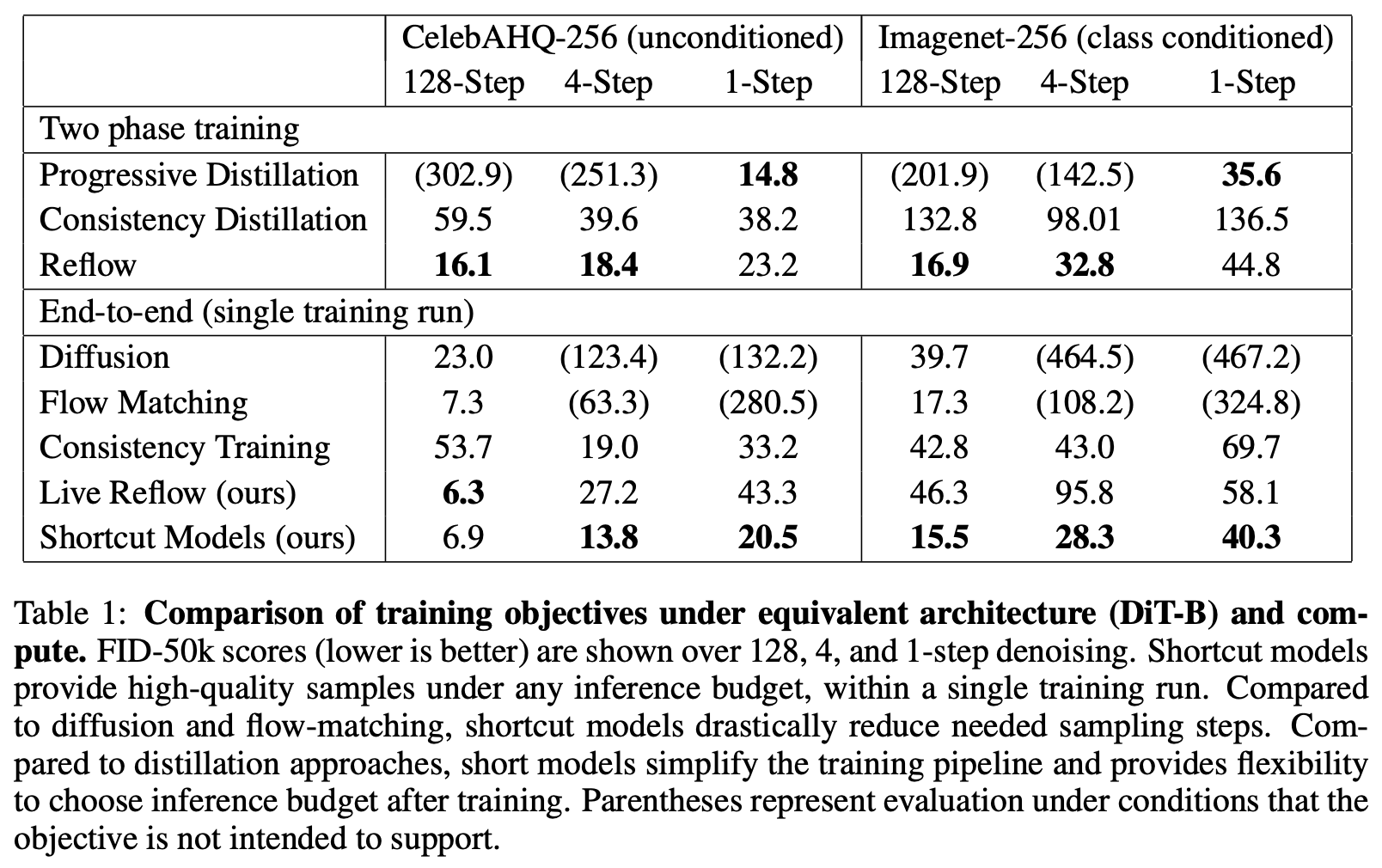
Now let’s look at the experimental results of the Shortcut Model. It appears to be the best-performing single-stage trained diffusion model for single-step generation currently available:
Here is the actual sampling effect:
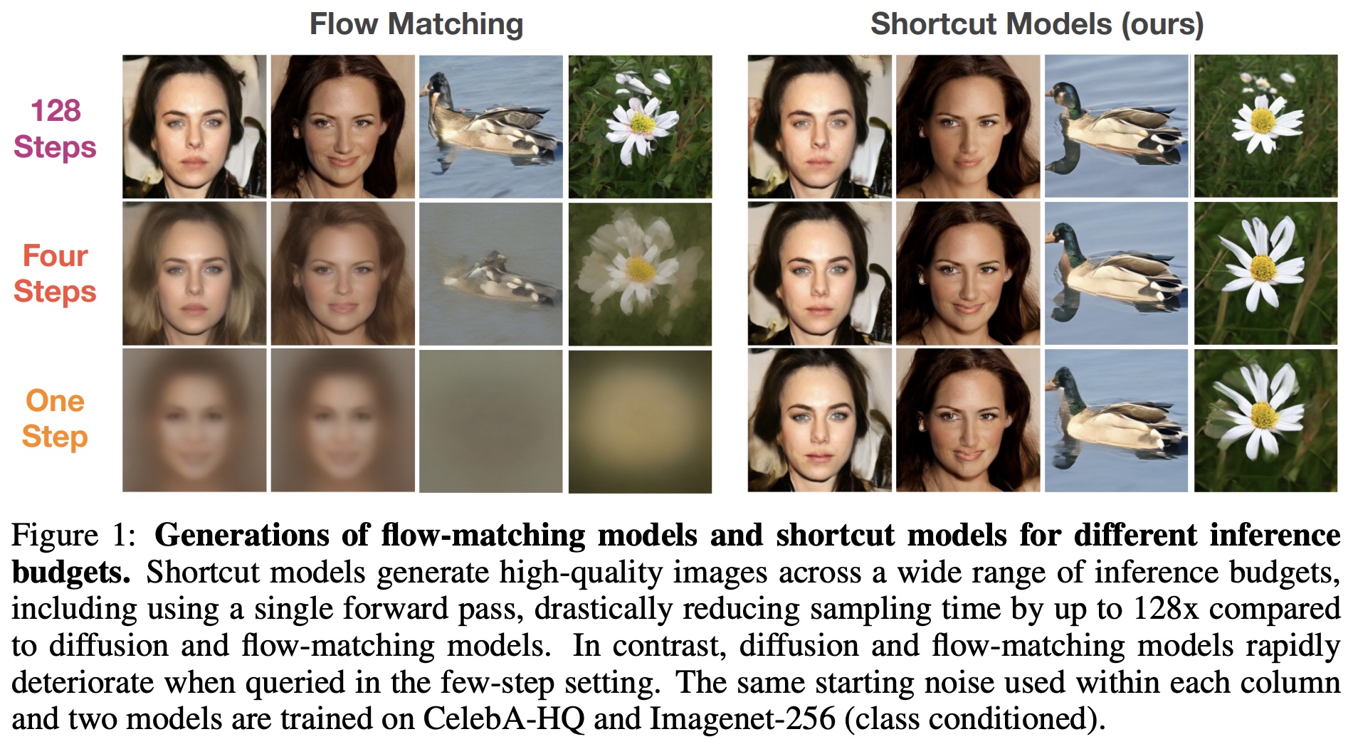
However, a close observation of the single-step generated samples reveals noticeable flaws. While the Shortcut Model has made significant progress compared to previous single-stage training schemes, there is still clear room for improvement.
The authors have open-sourced the code for the Shortcut Model. The GitHub link is:
Incidentally, the Shortcut Model was submitted to ICLR 2025 and received unanimous praise from reviewers (all scores of 8).
Extended Thinking
Seeing the Shortcut Model, what related works come to mind? One that might be unexpected is AMED, which we introduced in "Generative Diffusion Models (Part 21): Accelerating ODE Sampling with the Mean Value Theorem".
The underlying ideas of the Shortcut Model and AMED are connected. Both recognize that relying solely on complex high-order solvers to reduce the NFE (Number of Function Evaluations) to single digits is already difficult, let alone achieving single-step generation. Thus, they agree that what needs to change is not the solver, but the model itself. How should it change? AMED thought of the "Mean Value Theorem": by integrating both sides of the ODE, we have the exact: \boldsymbol{x}_{t + \epsilon} - \boldsymbol{x}_t = \int_t^{t + \epsilon}\boldsymbol{v}_{\boldsymbol{\theta}}(\boldsymbol{x}_{\tau}, \tau) d\tau By analogy with the Mean Value Theorem for Integrals, we can find an s \in [t, t + \epsilon] such that: \frac{1}{\epsilon}\int_t^{t + \epsilon}\boldsymbol{v}_{\boldsymbol{\theta}}(\boldsymbol{x}_{\tau}, \tau) d\tau = \boldsymbol{v}_{\boldsymbol{\theta}}(\boldsymbol{x}_s, s) Thus we get: \boldsymbol{x}_{t + \epsilon} - \boldsymbol{x}_t = \boldsymbol{v}_{\boldsymbol{\theta}}(\boldsymbol{x}_s, s) \epsilon Of course, the Mean Value Theorem for Integrals strictly applies only to scalar functions, not necessarily to vector functions, hence the "analogy." The problem is that the value of s is unknown, so AMED’s approach is to use a very small model (with negligible computation) to predict s.
AMED is a post-hoc correction method based on existing diffusion models, so its effectiveness depends on how well the Mean Value Theorem holds for the \boldsymbol{v}_{\boldsymbol{\theta}}(\boldsymbol{x}_t, t) model, which involves some "luck." Furthermore, AMED needs to use an Euler step to estimate \boldsymbol{x}_s first, so its minimum NFE is 2, and it cannot achieve single-step generation. In contrast, the Shortcut Model is more "aggressive"; it directly treats the step size as a conditional input and uses the acceleration condition [eq:cond] as a loss function. This not only avoids the feasibility discussion of the "Mean Value Theorem" approximation but also allows the minimum NFE to be reduced to 1.
More cleverly, upon closer reflection, we find commonalities in their approaches. As mentioned, Shortcut directly converts \epsilon into an Embedding and adds it to the Embedding of t. Isn’t this equivalent to modifying t, just as AMED does? The difference is that AMED directly modifies the numerical value of t, while Shortcut modifies the Embedding of t.
Summary
This article introduced a new work on diffusion models that achieves single-step generation through single-stage training. Its breakthrough idea is to treat the step size as a conditional input to the diffusion model, paired with an intuitive regularization term. This allows a single-step generation model to be obtained through a single stage of training.
Reprinting: Please include the original address of this article: https://kexue.fm/archives/10617
Further details on reprinting: Please refer to: "Scientific Space FAQ"