With the arrival of the LLM era, academic enthusiasm for optimizer research seems to have waned. This is primarily because the current mainstream AdamW already meets most needs, and "making major changes" to the optimizer requires enormous validation costs. Consequently, most current changes in optimizers are merely small patches applied to AdamW by the industry based on their own training experiences.
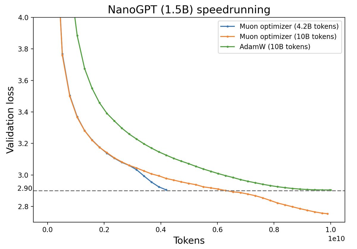
However, an optimizer named "Muon" has recently caused quite a stir on Twitter. It claims to be more efficient than AdamW and is not just a "minor tweak" on Adam; rather, it embodies some thought-provoking principles regarding the differences between vectors and matrices. In this article, let us appreciate it together.
Preliminary Algorithm Exploration
Muon stands for "MomentUm Orthogonalized by Newton-schulz". It is applicable to matrix parameters \boldsymbol{W}\in\mathbb{R}^{n\times m}, and its update rule is: \begin{aligned} \boldsymbol{M}_t &= \beta\boldsymbol{M}_{t-1} + \boldsymbol{G}_t \\[5pt] \boldsymbol{W}_t &= \boldsymbol{W}_{t-1} - \eta_t [\mathop{\mathrm{msign}}(\boldsymbol{M}_t) + \lambda \boldsymbol{W}_{t-1}] \\ \end{aligned} Here \mathop{\mathrm{msign}} is the matrix sign function. It is not a simple element-wise \mathop{\mathrm{sign}} operation on each component of the matrix, but a matrix-based generalization of the \mathop{\mathrm{sign}} function. Its relationship with SVD is: \boldsymbol{U},\boldsymbol{\Sigma},\boldsymbol{V}^{\top} = \text{SVD}(\boldsymbol{M}) \quad\Rightarrow\quad \mathop{\mathrm{msign}}(\boldsymbol{M}) = \boldsymbol{U}_{[:,:r]}\boldsymbol{V}_{[:,:r]}^{\top} where \boldsymbol{U}\in\mathbb{R}^{n\times n}, \boldsymbol{\Sigma}\in\mathbb{R}^{n\times m}, \boldsymbol{V}\in\mathbb{R}^{m\times m}, and r is the rank of \boldsymbol{M}. We will expand on more theoretical details later, but first, let’s try to intuitively perceive the following fact:
Muon is an adaptive learning rate optimizer similar to Adam.
Adaptive learning rate optimizers like Adagrad, RMSprop, and Adam are characterized by adjusting the update amount of each parameter by dividing by the square root of the moving average of the gradient squared. This achieves two effects: 1. Constant scaling of the loss function does not affect the optimization trajectory; 2. The update magnitude of each parameter component is as consistent as possible. Muon happens to satisfy these two characteristics:
If the loss function is multiplied by \lambda, \boldsymbol{M} will also be multiplied by \lambda. The result is that \boldsymbol{\Sigma} is multiplied by \lambda, but Muon’s final update amount turns \boldsymbol{\Sigma} into an identity matrix, so it does not affect the optimization result.
When \boldsymbol{M} is decomposed via SVD into \boldsymbol{U}\boldsymbol{\Sigma}\boldsymbol{V}^{\top}, the different singular values in \boldsymbol{\Sigma} reflect the "anisotropy" of \boldsymbol{M}. Setting them all to one makes the update more isotropic and serves to synchronize update magnitudes.
Regarding point 2, does any reader recall BERT-whitening? Additionally, it should be noted that Muon has a Nesterov version, which simply replaces \mathop{\mathrm{msign}}(\boldsymbol{M}_t) in the update rule with \mathop{\mathrm{msign}}(\beta\boldsymbol{M}_t + \boldsymbol{G}_t); the rest is identical. For simplicity, we won’t expand on it.
(Archaeology: It was later discovered that the 2015 paper "Stochastic Spectral Descent for Restricted Boltzmann Machines" had already proposed an optimization algorithm roughly identical to Muon, then called "Stochastic Spectral Descent".)
The Sign Function
Using SVD, we can also prove the identity: \mathop{\mathrm{msign}}(\boldsymbol{M}) = (\boldsymbol{M}\boldsymbol{M}^{\top})^{-1/2}\boldsymbol{M}= \boldsymbol{M}(\boldsymbol{M}^{\top}\boldsymbol{M})^{-1/2} \label{eq:msign-id} where {}^{-1/2} is the inverse of the matrix square root; if it is not invertible, the pseudo-inverse is taken. This identity helps us better understand why \mathop{\mathrm{msign}} is a matrix generalization of \mathop{\mathrm{sign}}: for a scalar x, we have \mathop{\mathrm{sign}}(x)=x(x^2)^{-1/2}, which is exactly a special case of the above formula (when \boldsymbol{M} is a 1\times 1 matrix). This special case can be extended to a diagonal matrix \boldsymbol{M}=\text{diag}(\boldsymbol{m}): \mathop{\mathrm{msign}}(\boldsymbol{M}) = \text{diag}(\boldsymbol{m})[\text{diag}(\boldsymbol{m})^2]^{-1/2} = \text{diag}(\mathop{\mathrm{sign}}(\boldsymbol{m}))=\mathop{\mathrm{sign}}(\boldsymbol{M}) where \mathop{\mathrm{sign}}(\boldsymbol{m}) and \mathop{\mathrm{sign}}(\boldsymbol{M}) refer to taking the \mathop{\mathrm{sign}} of each component of the vector/matrix. This means that when \boldsymbol{M} is a diagonal matrix, Muon degenerates into SignSGD (Signum) with momentum or Tiger proposed by the author, both of which are classic approximations of Adam. Conversely, the difference between Muon and Signum/Tiger is that the element-wise \mathop{\mathrm{sign}}(\boldsymbol{M}) is replaced by the matrix version \mathop{\mathrm{msign}}(\boldsymbol{M}).
For an n-dimensional vector, we can also view it as an n\times 1 matrix, in which case \mathop{\mathrm{msign}}(\boldsymbol{m}) = \boldsymbol{m}/\Vert\boldsymbol{m}\Vert_2 is exactly l_2 normalization. Thus, under the Muon framework, we have two perspectives for vectors: one is as a diagonal matrix (e.g., the gamma parameter in LayerNorm), resulting in taking the \mathop{\mathrm{sign}} of the momentum; the other is as an n\times 1 matrix, resulting in l_2 normalization of the momentum. Furthermore, although input and output Embeddings are matrices, they are used sparsely, so it is more reasonable to treat them as multiple independent vectors.
When m=n=r, \mathop{\mathrm{msign}}(\boldsymbol{M}) also has the meaning of the "optimal orthogonal approximation": \mathop{\mathrm{msign}}(\boldsymbol{M}) = \mathop{\mathrm{argmin}}_{\boldsymbol{O}^{\top}\boldsymbol{O} = \boldsymbol{I}}\Vert \boldsymbol{M} - \boldsymbol{O}\Vert_F^2 \label{eq:nearest-orth} Similarly, for \mathop{\mathrm{sign}}(\boldsymbol{M}), we can write (assuming \boldsymbol{M} has no zero elements): \mathop{\mathrm{sign}}(\boldsymbol{M}) = \mathop{\mathrm{argmin}}_{\boldsymbol{O}\in\{-1,1\}^{n\times m}}\Vert \boldsymbol{M} - \boldsymbol{O}\Vert_F^2 Whether it is \boldsymbol{O}^{\top}\boldsymbol{O} = \boldsymbol{I} or \boldsymbol{O}\in\{-1,1\}^{n\times m}, we can view this as a regularization constraint on the update amount. Therefore, Muon, Signum, and Tiger can be seen as optimizers under the same line of thought: they all start from momentum \boldsymbol{M} to construct the update amount, but choose different regularization methods for it.
Proof of Equation [eq:nearest-orth]: For an orthogonal matrix \boldsymbol{O}, we have \begin{aligned} \Vert \boldsymbol{M} - \boldsymbol{O}\Vert_F^2 &= \Vert \boldsymbol{M}\Vert_F^2 + \Vert \boldsymbol{O}\Vert_F^2 - 2\langle\boldsymbol{M},\boldsymbol{O}\rangle_F \\ &= \Vert \boldsymbol{M}\Vert_F^2 + n - 2\mathop{\mathrm{Tr}}(\boldsymbol{M}\boldsymbol{O}^{\top})\\ &= \Vert \boldsymbol{M}\Vert_F^2 + n - 2\mathop{\mathrm{Tr}}(\boldsymbol{U}\boldsymbol{\Sigma}\boldsymbol{V}^{\top}\boldsymbol{O}^{\top})\\ &= \Vert \boldsymbol{M}\Vert_F^2 + n - 2\mathop{\mathrm{Tr}}(\boldsymbol{\Sigma}\boldsymbol{V}^{\top}\boldsymbol{O}^{\top}\boldsymbol{U})\\ &= \Vert \boldsymbol{M}\Vert_F^2 + n - 2\sum_{i=1}^n \boldsymbol{\Sigma}_{i,i}(\boldsymbol{V}^{\top}\boldsymbol{O}^{\top}\boldsymbol{U})_{i,i} \end{aligned} The calculation rules involved were introduced in the article on pseudo-inverses. Since \boldsymbol{U}, \boldsymbol{V}, \boldsymbol{O} are all orthogonal matrices, \boldsymbol{V}^{\top}\boldsymbol{O}^{\top}\boldsymbol{U} is also an orthogonal matrix. Each component of an orthogonal matrix must not exceed 1. Since \boldsymbol{\Sigma}_{i,i} > 0, the minimum value of the above expression corresponds to taking the maximum value for each (\boldsymbol{V}^{\top}\boldsymbol{O}^{\top}\boldsymbol{U})_{i,i}, i.e., (\boldsymbol{V}^{\top}\boldsymbol{O}^{\top}\boldsymbol{U})_{i,i}=1. This implies \boldsymbol{V}^{\top}\boldsymbol{O}^{\top}\boldsymbol{U}=\boldsymbol{I}, or \boldsymbol{O}=\boldsymbol{U}\boldsymbol{V}^{\top}.
This conclusion can be carefully extended to cases where m, n, r are not equal, but we will not expand further here.
Iterative Solution
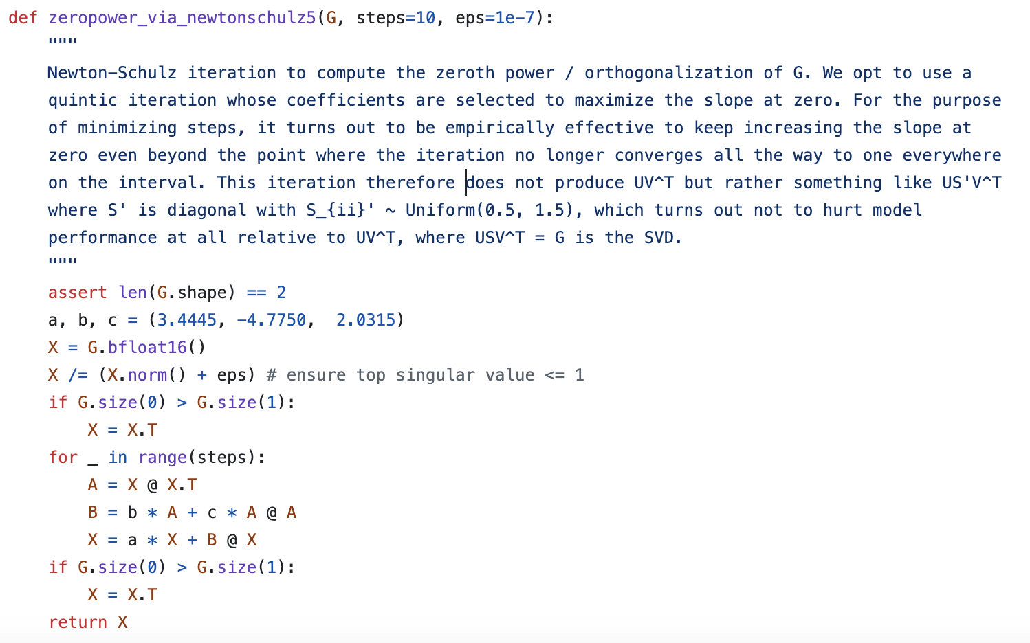
In practice, performing SVD at every step to solve for \mathop{\mathrm{msign}}(\boldsymbol{M}) would be computationally expensive. Therefore, the authors proposed using Newton-Schulz iteration to approximate \mathop{\mathrm{msign}}(\boldsymbol{M}).
The starting point for the iteration is the identity [eq:msign-id]. Without loss of generality, assume n \geq m, and consider the Taylor expansion of (\boldsymbol{M}^{\top}\boldsymbol{M})^{-1/2} at \boldsymbol{M}^{\top}\boldsymbol{M}=\boldsymbol{I}. The expansion is performed by applying the scalar function t^{-1/2} results directly to the matrix: t^{-1/2} = 1 - \frac{1}{2}(t-1) + \frac{3}{8}(t-1)^2 - \frac{5}{16}(t-1)^3 + \cdots Retaining up to the second order, the result is (15 - 10t + 3t^2)/8. Thus, we have: \mathop{\mathrm{msign}}(\boldsymbol{M}) = \boldsymbol{M}(\boldsymbol{M}^{\top}\boldsymbol{M})^{-1/2}\approx \frac{15}{8}\boldsymbol{M} - \frac{5}{4}\boldsymbol{M}(\boldsymbol{M}^{\top}\boldsymbol{M}) + \frac{3}{8}\boldsymbol{M}(\boldsymbol{M}^{\top}\boldsymbol{M})^2 If \boldsymbol{X}_t is an approximation of \mathop{\mathrm{msign}}(\boldsymbol{M}), substituting it into the above formula yields a better approximation. This gives us a usable iterative format: \boldsymbol{X}_{t+1} = \frac{15}{8}\boldsymbol{X}_t - \frac{5}{4}\boldsymbol{X}_t(\boldsymbol{X}_t^{\top}\boldsymbol{X}_t) + \frac{3}{8}\boldsymbol{X}_t(\boldsymbol{X}_t^{\top}\boldsymbol{X}_t)^2 However, checking the official Muon code reveals that while the Newton-Schulz iteration follows this form, the three coefficients are (3.4445, -4.7750, 2.0315). The author did not provide a mathematical derivation, only a somewhat vague comment:
Convergence Acceleration
To guess the source of the official iteration algorithm, we consider a general iteration process: \boldsymbol{X}_{t+1} = a\boldsymbol{X}_t + b\boldsymbol{X}_t(\boldsymbol{X}_t^{\top}\boldsymbol{X}_t) + c\boldsymbol{X}_t(\boldsymbol{X}_t^{\top}\boldsymbol{X}_t)^2 \label{eq:iteration} where a, b, c are three coefficients to be solved. If a higher-order iteration algorithm is desired, one could sequentially add terms like \boldsymbol{X}_t(\boldsymbol{X}_t^{\top}\boldsymbol{X}_t)^3, etc.
We choose the initial value \boldsymbol{X}_0 = \boldsymbol{M}/\Vert\boldsymbol{M}\Vert_F. Dividing by the Frobenius norm does not change the SVD’s \boldsymbol{U}, \boldsymbol{V} but ensures all singular values of \boldsymbol{X}_0 are in [0, 1]. Assuming \boldsymbol{X}_t can be decomposed as \boldsymbol{U}\boldsymbol{\Sigma}_t\boldsymbol{V}^{\top}, substituting into the iteration gives: \boldsymbol{X}_{t+1} = \boldsymbol{U}_{[:,:r]}(a \boldsymbol{\Sigma}_{t,[:r,:r]} + b \boldsymbol{\Sigma}_{t,[:r,:r]}^3 + c \boldsymbol{\Sigma}_{t,[:r,:r]}^5)\boldsymbol{V}_{[:,:r]}^{\top} Thus, the iteration effectively acts on the singular values. Let g(x) = ax + bx^3 + cx^5. The goal is to iterate \sigma_{t+1} = g(\sigma_t) such that singular values converge to 1.
Inspired by @leloykun, we treat the selection of a, b, c as an optimization problem to make the iteration converge as fast as possible for any initial singular value. We re-parameterize g(x) as: g(x) = x + \kappa x(x^2 - x_1^2)(x^2 - x_2^2) where x_1 \leq x_2. This identifies fixed points at 0, \pm x_1, \pm x_2. By sampling matrices, calculating singular values via SVD, and using gradient descent to minimize the squared error from 1 after T steps, we can find optimal coefficients.
| n | m | T | \kappa | x_1 | x_2 | a | b | c | mse | mse_o |
|---|---|---|---|---|---|---|---|---|---|---|
| 1024 | 1024 | 3 | 7.020 | 0.830 | 0.830 | 4.328 | -9.666 | 7.020 | 0.10257 | 0.18278 |
| 1024 | 1024 | 5 | 1.724 | 0.935 | 1.235 | 3.297 | -4.136 | 1.724 | 0.02733 | 0.04431 |
| 2048 | 1024 | 3 | 7.028 | 0.815 | 0.815 | 4.095 | -9.327 | 7.028 | 0.01628 | 0.06171 |
| 2048 | 1024 | 5 | 1.476 | 0.983 | 1.074 | 2.644 | -3.128 | 1.476 | 0.00038 | 0.02954 |
| 4096 | 1024 | 3 | 6.948 | 0.802 | 0.804 | 3.886 | -8.956 | 6.948 | 0.00371 | 0.02574 |
| 4096 | 1024 | 5 | 1.214 | 1.047 | 1.048 | 2.461 | -2.663 | 1.214 | 0.00008 | 0.02563 |
| 2048 | 2048 | 3 | 11.130 | 0.767 | 0.767 | 4.857 | -13.103 | 11.130 | 0.10739 | 0.24410 |
| 2048 | 2048 | 5 | 1.779 | 0.921 | 1.243 | 3.333 | -4.259 | 1.779 | 0.03516 | 0.04991 |
Here mse_o is the result using the Muon author’s coefficients. The author’s a, b, c roughly correspond to the optimal solution for square matrices with T=5.
Reference code:
import jax
import jax.numpy as jnp
from tqdm import tqdm

n, m, T = 1024, 1024, 5
key, data = jax.random.key(42), jnp.array([])
for _ in tqdm(range(1000), ncols=0, desc='SVD'):
    key, subkey = jax.random.split(key)
    M = jax.random.normal(subkey, shape=(n, m))
    S = jnp.linalg.svd(M, full_matrices=False)[1]
    data = jnp.concatenate([data, S / (S**2).sum()**0.5])

@jax.jit
def f(w, x):
    k, x1, x2 = w
    for _ in range(T):
        x = x + k * x * (x**2 - x1**2) * (x**2 - x2**2)
    return ((x - 1)**2).mean()

f_grad = jax.grad(f)
w, u = jnp.array([1, 0.9, 1.1]), jnp.zeros(3)
for _ in tqdm(range(100000), ncols=0, desc='SGD'):
    u = 0.9 * u + f_grad(w, data)
    w = w - 0.01 * u

k, x1, x2 = w
a, b, c = 1 + k * x1**2 * x2**2, -k * (x1**2 + x2**2), k
print(f'{n} & {m} & {T} & {k:.3f} & {x1:.3f} & {x2:.3f} & {a:.3f} & {b:.3f} & {c:.3f} & {f(w, data):.5f}')
Some Thoughts
If T=5 is chosen, Muon requires 15 matrix multiplications per step for an n \times n matrix. While this is more than Adam, the overhead is small (within 2-5%) because these operations occur when the GPU would otherwise be idle between gradient computations.
The most profound aspect of Muon is the distinction between vectors and matrices. Standard optimizers are element-wise, treating everything as a large vector. Muon treats matrices as fundamental units, respecting properties like the "trace" or "eigenvalues" which are invariant under similarity transformations. This non-element-wise approach captures the essential differences but introduces challenges for tensor parallelism, as gradients must be aggregated before the update.
Norm Perspective
What key property does Muon capture? The norm perspective provides an answer. Following the logic of "steepest descent" under a norm constraint: \Delta\boldsymbol{w}_{t+1} = \mathop{\mathrm{argmin}}_{\Delta\boldsymbol{w}} \frac{\Vert\Delta\boldsymbol{w}\Vert^2}{2\eta_t} + \boldsymbol{g}_t^{\top}\Delta\boldsymbol{w} For the l_2 norm, this yields SGD. For the l_\infty norm, it yields SignSGD.
Matrix Norms
For matrix parameters \boldsymbol{W}, if we use the Frobenius norm, we get SGD. However, if we use the spectral norm (2-norm): \Vert \boldsymbol{\Phi}\Vert_2 = \max_{\Vert \boldsymbol{x}\Vert_2 = 1} \Vert \boldsymbol{\Phi}\boldsymbol{x}\Vert_2 It can be shown that the update direction \boldsymbol{\Phi} that maximizes \mathop{\mathrm{Tr}}(\boldsymbol{G}^{\top}\boldsymbol{\Phi}) subject to \Vert \boldsymbol{\Phi}\Vert_2 = 1 is exactly \mathop{\mathrm{msign}}(\boldsymbol{G}). Thus, Muon is steepest descent under the spectral norm constraint.
Tracing the Roots
Muon is related to Shampoo (2018), which uses \boldsymbol{L}_t^{-1/4}\boldsymbol{G}_t\boldsymbol{R}_t^{-1/4} for updates. When the momentum factor \beta=0, Shampoo’s update is theoretically equivalent to \mathop{\mathrm{msign}}(\boldsymbol{G}), showing that Muon and Shampoo share a common lineage in update design.
Summary
This article introduced the Muon optimizer, customized for matrix parameters. It appears more efficient than AdamW and highlights the fundamental differences between vector and matrix optimization.
Reprinting: Please include the original link: https://kexue.fm/archives/10592