In the previous article "How should the learning rate change when the Batch Size increases?", we discussed the scaling laws between learning rate and batch size from multiple perspectives. For the Adam optimizer, we employed the SignSGD approximation, which is a common technique for analyzing Adam. A natural question then arises: how scientifically sound is it to approximate Adam with SignSGD?
We know that the denominator of the Adam optimizer’s update includes an \epsilon. Its original purpose was to prevent division-by-zero errors, so its value is typically very close to zero—so much so that we usually ignore it in theoretical analyses. However, in current Large Language Model (LLM) training, especially with low-precision training, we often choose a relatively large \epsilon. This leads to a situation where, in the middle and late stages of training, \epsilon often exceeds the magnitude of the squared gradient. Therefore, the existence of \epsilon is, in fact, no longer negligible.
In this article, we attempt to explore how \epsilon affects the Scaling Law of Adam’s learning rate and batch size, providing a reference calculation scheme for related issues.
SoftSign
Since this is a continuation of the previous article, I will not repeat the relevant background. To investigate the role of \epsilon, we switch from SignSGD to SoftSignSGD. That is, \tilde{\boldsymbol{\varphi}}_B = \mathop{\mathrm{sign}}(\tilde{\boldsymbol{g}}_B) becomes \tilde{\boldsymbol{\varphi}}_B = \text{softsign}(\tilde{\boldsymbol{g}}_B, \epsilon), where: \mathop{\mathrm{sign}}(x)=\frac{x}{\sqrt{x^2}} \quad \to \quad \text{softsign}(x, \epsilon)=\frac{x}{\sqrt{x^2+\epsilon^2}} This form is undoubtedly closer to Adam. But before proceeding, we need to confirm whether \epsilon is truly non-negligible to determine if further research is worthwhile.
In the Keras implementation of Adam, the default value of \epsilon is 10^{-7}, and in Torch, it is 10^{-8}. At these levels, the probability of the absolute value of the gradient being smaller than \epsilon is not very high. However, in LLMs, a common value for \epsilon is 10^{-5} (e.g., in LLAMA2). Once training enters the "normal" phase, components where the absolute value of the gradient is smaller than \epsilon become very common, so the impact of \epsilon is significant.
This is also related to the number of parameters in the LLM. For a model that can be trained stably, regardless of its parameter count, the magnitude of its gradient norm is roughly in the same order of magnitude, which is determined by the stability of backpropagation (refer to "What are the difficulties in training a 1000-layer Transformer?"). Therefore, for models with more parameters, the average absolute value of the gradient for each parameter becomes relatively smaller, making the role of \epsilon more prominent.
It is worth noting that the introduction of \epsilon actually provides an interpolation between Adam and SGD. This is because when x \neq 0: \lim_{\epsilon\to \infty}\epsilon\,\text{softsign}(x, \epsilon)=\lim_{\epsilon\to \infty}\frac{x \epsilon}{\sqrt{x^2+\epsilon^2}} = x Thus, the larger the \epsilon, the more Adam behaves like SGD.
S-shaped Approximation
Having confirmed the necessity of introducing \epsilon, we begin our analysis. During the process, we will repeatedly encounter S-shaped functions, so a preparatory task is to explore simple approximations for them.
S-shaped functions are quite common; the \text{softsign} function introduced in the previous section is one, and the \text{erf} function used in the previous article is another. Others include \tanh and \text{sigmoid}. We are dealing with S-shaped functions S(x) that satisfy the following properties:
1. Globally smooth and monotonically increasing;
2. Odd function with a range of [-1, 1];
3. Slope at the origin is k > 0.
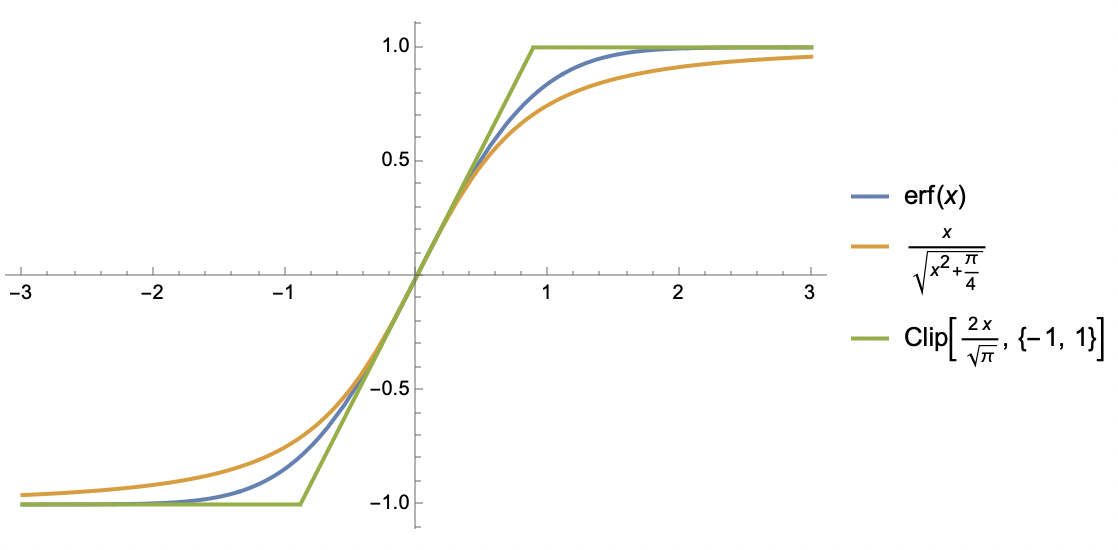
For such functions, we consider two approximations. The first is similar to \text{softsign}: S(x)\approx \frac{x}{\sqrt{x^2 + 1/k^2}} This is perhaps the simplest function that preserves the three properties mentioned above. The second approximation is based on the \text{clip} function: S(x)\approx \text{clip}(kx, -1, 1) \triangleq \left\{\begin{aligned}&1, &kx\geq 1 \\ &kx, & -1 < kx < 1\\ &-1, &kx \leq -1\end{aligned}\right. This is essentially a piecewise linear function. It sacrifices global smoothness, but piecewise linearity makes integration much easier, as we will soon see.
Mean Estimation
Following the method of the previous article, our starting point is: \mathbb{E}[\mathcal{L}(\boldsymbol{w} - \eta\tilde{\boldsymbol{\varphi}}_B)] \approx \mathcal{L}(\boldsymbol{w}) - \eta\mathbb{E}[\tilde{\boldsymbol{\varphi}}_B]^{\top}\boldsymbol{g} + \frac{1}{2}\eta^2 \text{Tr}(\mathbb{E}[\tilde{\boldsymbol{\varphi}}_B\tilde{\boldsymbol{\varphi}}_B^{\top}]\boldsymbol{H}) We need to estimate \mathbb{E}[\tilde{\boldsymbol{\varphi}}_B] and \mathbb{E}[\tilde{\boldsymbol{\varphi}}_B\tilde{\boldsymbol{\varphi}}_B^{\top}].
In this section, we calculate \mathbb{E}[\tilde{\boldsymbol{\varphi}}_B]. To do this, we use the \text{clip} function to approximate the \text{softsign} function: \text{softsign}(x, \epsilon)\approx \text{clip}(x/\epsilon, -1, 1) = \left\{\begin{aligned}&1, & x/\epsilon \geq 1 \\ & x / \epsilon, & -1 < x/\epsilon < 1 \\ &-1, & x/\epsilon \leq -1 \\ \end{aligned}\right. Then we have: \begin{aligned} \mathbb{E}[\tilde{\varphi}_B] =&\, \mathbb{E}[\text{softsign}(g + \sigma z/\sqrt{B}, \epsilon)] \approx \mathbb{E}[\text{clip}(g/\epsilon + \sigma z/\epsilon\sqrt{B},-1, 1)] \\[5pt] =&\,\frac{1}{\sqrt{2\pi}}\int_{-\infty}^{\infty} \text{clip}(g/\epsilon + \sigma z/\epsilon\sqrt{B},-1, 1) e^{-z^2/2}dz \\[5pt] =&\,\frac{1}{\sqrt{2\pi}}\int_{-\infty}^{-(g+\epsilon)\sqrt{B}/\sigma} (-1)\times e^{-z^2/2}dz + \frac{1}{\sqrt{2\pi}}\int_{-(g-\epsilon)\sqrt{B}/\sigma}^{\infty} 1\times e^{-z^2/2}dz \\[5pt] & \quad + \frac{1}{\sqrt{2\pi}}\int_{-(g+\epsilon)\sqrt{B}/\sigma}^{-(g-\epsilon)\sqrt{B}/\sigma} (g/\epsilon + \sigma z/\epsilon\sqrt{B})\times e^{-z^2/2}dz \end{aligned} The integral form is complex, but calculating it with Mathematica is not difficult. The result can be expressed using the \text{erf} function: \frac{1}{2}\left[\mathop{\mathrm{erf}}\left(\frac{a+b}{\sqrt{2}}\right)+\mathop{\mathrm{erf}}\left(\frac{a-b}{\sqrt{2}}\right)\right]+\frac{a}{2b}\left[\mathop{\mathrm{erf}}\left(\frac{a+b}{\sqrt{2}}\right)-\mathop{\mathrm{erf}}\left(\frac{a-b}{\sqrt{2}}\right)\right]+\frac{e^{-(a+b)^2/2} - e^{-(a-b)^2/2}}{b\sqrt{2\pi}} where a = g\sqrt{B}/\sigma, b=\epsilon \sqrt{B}/\sigma. Although this function looks complicated, it is an S-shaped function of a, with a range of (-1, 1) and a slope at a=0 of \mathop{\mathrm{erf}}(b/\sqrt{2})/b. Using the first approximation form: \mathbb{E}[\tilde{\varphi}_B]\approx\frac{a}{\sqrt{a^2 + b^2 / \mathop{\mathrm{erf}}(b/\sqrt{2})^2}}\approx \frac{a}{\sqrt{a^2 + b^2 + \pi / 2}}=\frac{g/\sigma}{\sqrt{(g^2+\epsilon^2)/\sigma^2 + \pi / 2B}} \label{eq:E-u-approx} The second approximation uses \mathop{\mathrm{erf}}(x)\approx x / \sqrt{x^2 + \pi / 4} to handle the \mathop{\mathrm{erf}}(b/\sqrt{2}) in the denominator. Fortunately, the final form is not too complex. Next, we have: \mathbb{E}[\tilde{\boldsymbol{\varphi}}_B]_i \approx \frac{g_i/\sigma_i}{\sqrt{(g_i^2+\epsilon^2)/\sigma_i^2 + \pi / 2B}} = \frac{\text{softsign}(g_i, \epsilon)}{\sqrt{1 + \pi \sigma_i^2 /(g_i^2+\epsilon^2)/2B}}\approx \frac{\text{softsign}(g_i, \epsilon)}{\sqrt{1 + \pi \kappa^2/2B}} = \nu_i \beta As in the previous article, the last approximation uses a mean-field approach, where \kappa^2 is some average of all \sigma_i^2 /(g_i^2+\epsilon^2), \nu_i = \text{softsign}(g_i, \epsilon), and \beta = (1 + \pi\kappa^2 / 2B)^{-1/2}.
Variance Estimation
The first moment is solved; now it is the turn of the second moment: \begin{aligned} \mathbb{E}[\tilde{\varphi}_B^2] =&\, \mathbb{E}[\text{softsign}(g + \sigma z/\sqrt{B}, \epsilon)^2] \approx \mathbb{E}[\text{clip}(g/\epsilon + \sigma z/\epsilon\sqrt{B},-1, 1)^2] \\[5pt] =&\,\frac{1}{\sqrt{2\pi}}\int_{-\infty}^{\infty} \text{clip}(g/\epsilon + \sigma z/\epsilon\sqrt{B},-1, 1)^2 e^{-z^2/2}dz \\[5pt] =&\,\frac{1}{\sqrt{2\pi}}\int_{-\infty}^{-(g+\epsilon)\sqrt{B}/\sigma} (-1)^2\times e^{-z^2/2}dz + \frac{1}{\sqrt{2\pi}}\int_{-(g-\epsilon)\sqrt{B}/\sigma}^{\infty} 1^2\times e^{-z^2/2}dz \\[5pt] & \quad + \frac{1}{\sqrt{2\pi}}\int_{-(g+\epsilon)\sqrt{B}/\sigma}^{-(g-\epsilon)\sqrt{B}/\sigma} (g/\epsilon + \sigma z/\epsilon\sqrt{B})^2\times e^{-z^2/2}dz \end{aligned} The result can also be expressed with the \mathop{\mathrm{erf}} function but is even more lengthy. When viewed as a function of a, the result is an inverted bell-shaped curve, symmetric about the y-axis, with an upper bound of 1 and a minimum value in (0, 1). Referring to the approximation of \mathbb{E}[\tilde{\varphi}_B] in Eq. [eq:E-u-approx], we choose the following approximation: \mathbb{E}[\tilde{\varphi}_B^2] \approx 1 - \frac{b^2}{a^2 + b^2 + \pi / 2} = 1 - \frac{\epsilon^2/(g^2+\epsilon^2)}{1 + \pi\sigma^2/(g^2+\epsilon^2) / 2B} To be honest, the accuracy of this approximation is not very high; it is mainly for computational convenience. However, it preserves key characteristics: inverted bell shape, y-axis symmetry, upper bound of 1, result of 1 when b=0, and result of 0 as b \to \infty. Continuing with the mean-field approximation: \mathbb{E}[\tilde{\boldsymbol{\varphi}}_B\tilde{\boldsymbol{\varphi}}_B^{\top}]_{i,i} \approx 1 - \frac{\epsilon^2/(g_i^2+\epsilon^2)}{1 + \pi\sigma_i^2/(g_i^2+\epsilon^2) / 2B}\approx 1 - \frac{\epsilon^2/(g_i^2+\epsilon^2)}{1 + \pi\kappa^2 / 2B} = \nu_i^2 \beta^2 + (1 - \beta^2) Thus \mathbb{E}[\tilde{\boldsymbol{\varphi}}_B\tilde{\boldsymbol{\varphi}}_B^{\top}]_{i,j}\approx \nu_i \nu_j \beta^2 + \delta_{i,j}(1-\beta^2). The term \delta_{i,j}(1-\beta^2) represents the covariance matrix of \tilde{\boldsymbol{\varphi}}, which is (1-\beta^2)\boldsymbol{I}. This diagonal matrix is expected because one of our assumptions is the independence between the components of \tilde{\boldsymbol{\varphi}}.
Initial Results
From this, we obtain: \eta^* \approx \frac{\mathbb{E}[\tilde{\boldsymbol{\varphi}}_B]^{\top}\boldsymbol{g}}{\text{Tr}(\mathbb{E}[\tilde{\boldsymbol{\varphi}}_B\tilde{\boldsymbol{\varphi}}_B^{\top}]\boldsymbol{H})} \approx \frac{\beta\sum_i \nu_i g_i}{\beta^2\sum_{i,j} \nu_i \nu_j H_{i,j} + (1-\beta^2)\sum_i H_{i,i} } Note that except for \beta, none of the other symbols depend on B, so the above equation already gives the dependency of \eta^* on B. To ensure the existence of a minimum, we assume the positive definiteness of the Hessian matrix \boldsymbol{H}, which implies \sum_{i,j} \nu_i \nu_j H_{i,j} > 0 and \sum_i H_{i,i} > 0.
In the previous article, we mentioned that the most important characteristic of Adam is the possible occurrence of the "Surge phenomenon," where \eta^* is no longer a globally monotonically increasing function of B. We will now prove that the introduction of \epsilon > 0 reduces the probability of the Surge phenomenon and that it disappears entirely as \epsilon \to \infty. The proof is straightforward: a necessary condition for the Surge phenomenon is: \sum_{i,j} \nu_i \nu_j H_{i,j} - \sum_i H_{i,i} > 0 If this is not true, \eta^* is monotonically increasing with respect to \beta, and since \beta is monotonically increasing with B, \eta^* is monotonically increasing with B, and no Surge phenomenon occurs. Recall that \nu_i = \text{softsign}(g_i, \epsilon) is a monotonically decreasing function of \epsilon. Therefore, as \epsilon increases, \sum_{i,j} \nu_i \nu_j H_{i,j} becomes smaller, making the above inequality less likely to hold. As \epsilon \to \infty, \nu_i tends to zero, the inequality cannot hold, and the Surge phenomenon disappears.
Furthermore, we can prove that as \epsilon \to \infty, the result is consistent with SGD. We only need to note that: \frac{\eta^*}{\epsilon} \approx \frac{\beta\sum_i (\epsilon \nu_i) g_i}{\beta^2\sum_{i,j} (\epsilon \nu_i)(\epsilon \nu_j) H_{i,j} + \epsilon^2(1-\beta^2)\sum_i H_{i,i} } We have the limits: \lim_{\epsilon\to\infty} \beta = 1,\quad\lim_{\epsilon\to\infty} \epsilon \nu_i = g_i, \quad \lim_{\epsilon\to\infty} \epsilon^2(1-\beta^2) = \pi \sigma^2 / 2B Here \sigma^2 is some average of all \sigma_i^2. Thus, when \epsilon is large enough, we have the approximation: \frac{\eta^*}{\epsilon} \approx \frac{\sum_i g_i^2}{\sum_{i,j} g_i g_j H_{i,j} + \left(\pi \sigma^2\sum_i H_{i,i}\right)/2B } The right side is the SGD result assuming the gradient covariance matrix is (\pi\sigma^2/2B)\boldsymbol{I}.
Summary
This article continues the methodology of the previous one, attempting to analyze the impact of Adam’s \epsilon on the Scaling Law between learning rate and Batch Size. The result is a form that lies between SGD and SignSGD. As \epsilon increases, the result becomes closer to SGD, and the probability of the "Surge phenomenon" decreases. Overall, the calculation results are not particularly surprising, but they serve as a reference process for analyzing the role of \epsilon.
Original address: https://kexue.fm/archives/10563