In the previous article, we introduced the “pseudo-inverse,” which relates to the optimal solution of the objective \Vert \boldsymbol{A}\boldsymbol{B} - \boldsymbol{M}\Vert_F^2 given matrices \boldsymbol{M} and \boldsymbol{A} (or \boldsymbol{B}). In this article, we focus on the optimal solution when neither \boldsymbol{A} nor \boldsymbol{B} is given, namely: \mathop{\text{argmin}}_{\boldsymbol{A},\boldsymbol{B}}\Vert \boldsymbol{A}\boldsymbol{B} - \boldsymbol{M}\Vert_F^2\label{eq:loss-ab} where \boldsymbol{A}\in\mathbb{R}^{n\times r}, \boldsymbol{B}\in\mathbb{R}^{r\times m}, \boldsymbol{M}\in\mathbb{R}^{n\times m}, r < \min(n,m). Simply put, this is about finding the “optimal r-rank approximation (the best approximation with rank not exceeding r)” of the matrix \boldsymbol{M}. To solve this problem, we need to introduce the famous “SVD (Singular Value Decomposition).” Although this series began with the pseudo-inverse, its fame is far less than that of SVD. There are likely many who have heard of or even used SVD but have never heard of the pseudo-inverse; the author himself learned about SVD before encountering the pseudo-inverse.
Next, we will introduce SVD around the concept of the optimal low-rank approximation of a matrix.
A First Look at the Conclusions
For any matrix \boldsymbol{M}\in\mathbb{R}^{n\times m}, one can find a Singular Value Decomposition (SVD) of the following form: \boldsymbol{M} = \boldsymbol{U}\boldsymbol{\Sigma} \boldsymbol{V}^{\top} where \boldsymbol{U}\in\mathbb{R}^{n\times n} and \boldsymbol{V}\in\mathbb{R}^{m\times m} are both orthogonal matrices, and \boldsymbol{\Sigma}\in\mathbb{R}^{n\times m} is a non-negative diagonal matrix: \boldsymbol{\Sigma}_{i,j} = \left\{\begin{aligned}&\sigma_i, &i = j \\ &0,&i \neq j\end{aligned}\right. The diagonal elements are sorted by default from largest to smallest, i.e., \sigma_1\geq \sigma_2\geq\sigma_3\geq\cdots\geq 0. These diagonal elements are called Singular Values. From a numerical computation perspective, we can retain only the non-zero elements in \boldsymbol{\Sigma}, reducing the sizes of \boldsymbol{U}, \boldsymbol{\Sigma}, \boldsymbol{V} to n\times r, r\times r, m\times r (where r is the rank of \boldsymbol{M}). Retaining the full orthogonal matrices is more convenient for theoretical analysis.
SVD also holds for complex matrices, but orthogonal matrices must be replaced by unitary matrices, and the transpose by the conjugate transpose. However, here we focus primarily on real matrix results, which are more closely related to machine learning. The fundamental theory of SVD includes its existence, calculation methods, and its connection to the optimal low-rank approximation. I will provide my own understanding of these topics later.
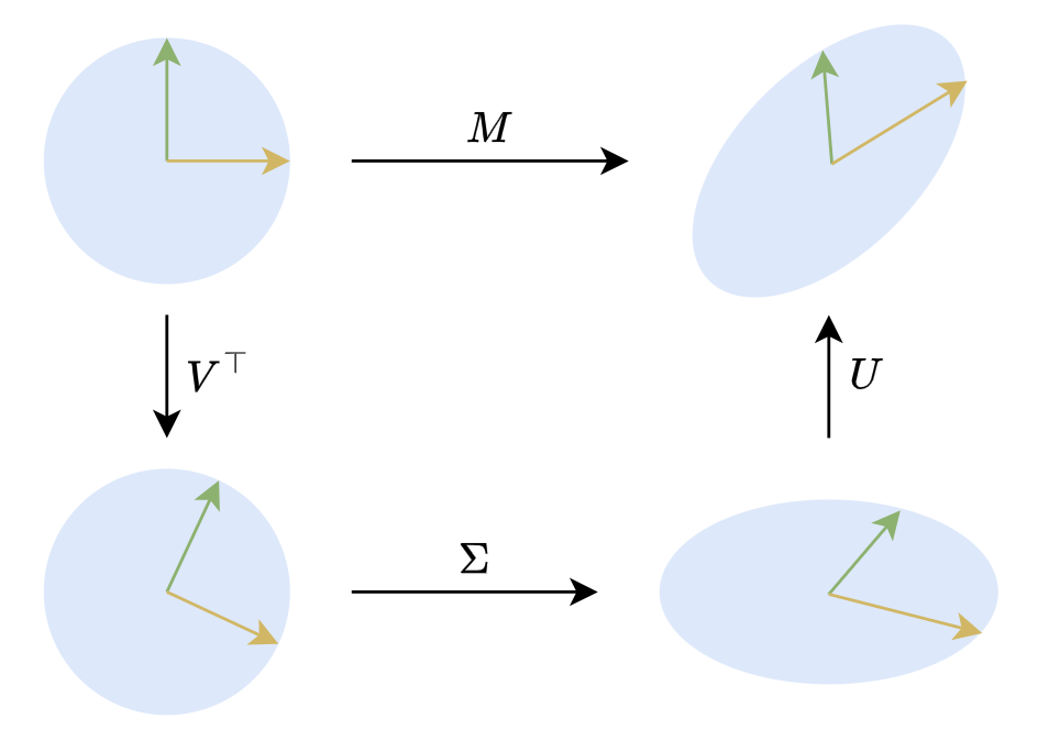
In a two-dimensional plane, SVD has a very intuitive geometric meaning. A two-dimensional orthogonal matrix mainly represents rotation (and reflection, but for geometric intuition, we can be less rigorous). Therefore, \boldsymbol{M}\boldsymbol{x}=\boldsymbol{U}\boldsymbol{\Sigma} \boldsymbol{V}^{\top}\boldsymbol{x} means that any linear transformation of a (column) vector \boldsymbol{x} can be decomposed into three steps: rotation, stretching, and rotation, as shown in the figure below:
Some Applications
Whether in theoretical analysis or numerical computation, SVD has very wide applications. One of the underlying principles is that commonly used matrix/vector norms are invariant under orthogonal transformations. Thus, the characteristic of SVD—having two orthogonal matrices sandwiching a diagonal matrix—often allows many matrix-related optimization objectives to be converted into equivalent cases involving non-negative diagonal matrices, thereby simplifying the problem.
General Solution for the Pseudo-inverse
Taking the pseudo-inverse as an example, when \boldsymbol{A}\in\mathbb{R}^{n\times r} has rank r, we have: \boldsymbol{A}^{\dagger} = \mathop{\text{argmin}}_{\boldsymbol{B}\in\mathbb{R}^{r\times n}}\Vert \boldsymbol{A}\boldsymbol{B} - \boldsymbol{I}_n\Vert_F^2 In the previous article, we derived the expression for \boldsymbol{A}^{\dagger} by taking derivatives and then spent some effort generalizing it to cases where the rank of \boldsymbol{A} is less than r. However, if we introduce SVD, the problem becomes much simpler. We can decompose \boldsymbol{A} into \boldsymbol{U}\boldsymbol{\Sigma} \boldsymbol{V}^{\top} and then represent \boldsymbol{B} as \boldsymbol{V} \boldsymbol{Z} \boldsymbol{U}^{\top}. Note that we do not require \boldsymbol{Z} to be diagonal, so \boldsymbol{B}=\boldsymbol{V} \boldsymbol{Z} \boldsymbol{U}^{\top} can always be achieved. Thus: \begin{aligned} \min_{\boldsymbol{B}}\Vert \boldsymbol{A}\boldsymbol{B} - \boldsymbol{I}_n\Vert_F^2 =&\, \min_{\boldsymbol{Z}}\Vert \boldsymbol{U}\boldsymbol{\Sigma} \boldsymbol{V}^{\top}\boldsymbol{V} \boldsymbol{Z} \boldsymbol{U}^{\top} - \boldsymbol{I}_n\Vert_F^2 \\ =&\, \min_{\boldsymbol{Z}}\Vert \boldsymbol{U}(\boldsymbol{\Sigma} \boldsymbol{Z} - \boldsymbol{I}_n) \boldsymbol{U}^{\top}\Vert_F^2 \\ =&\, \min_{\boldsymbol{Z}}\Vert \boldsymbol{\Sigma} \boldsymbol{Z} - \boldsymbol{I}_n\Vert_F^2 \end{aligned} The last equality is based on the conclusion we proved in the previous article: “orthogonal transformations do not change the F-norm.” This simplifies the problem to the pseudo-inverse of the diagonal matrix \boldsymbol{\Sigma}. We can then use block matrix form to represent \boldsymbol{\Sigma} \boldsymbol{Z} - \boldsymbol{I}_n as: \begin{aligned}\boldsymbol{\Sigma} \boldsymbol{Z} - \boldsymbol{I}_n =&\, \begin{pmatrix}\boldsymbol{\Sigma}_{[:r,:r]} \\ \boldsymbol{0}_{(n-r)\times r}\end{pmatrix} \begin{pmatrix}\boldsymbol{Z}_{[:r,:r]} & \boldsymbol{Z}_{[:r,r:]}\end{pmatrix} - \begin{pmatrix}\boldsymbol{I}_r & \boldsymbol{0}_{r\times(n-r)} \\ \boldsymbol{0}_{(n-r)\times r} & \boldsymbol{I}_{n-r}\end{pmatrix} \\ =&\, \begin{pmatrix}\boldsymbol{\Sigma}_{[:r,:r]}\boldsymbol{Z}_{[:r,:r]} - \boldsymbol{I}_r & \boldsymbol{\Sigma}_{[:r,:r]}\boldsymbol{Z}_{[:r,r:]}\\ \boldsymbol{0}_{(n-r)\times r} & -\boldsymbol{I}_{n-r}\end{pmatrix} \end{aligned} The slicing here follows the rules of Python arrays. From the final form, it is clear that to minimize the F-norm of \boldsymbol{\Sigma} \boldsymbol{Z} - \boldsymbol{I}_n, the unique solution is \boldsymbol{Z}_{[:r,:r]}=\boldsymbol{\Sigma}_{[:r,:r]}^{-1} and \boldsymbol{Z}_{[:r,r:]}=\boldsymbol{0}_{r\times(n-r)}. In plain terms, \boldsymbol{Z} is obtained by taking the reciprocal of the non-zero elements of \boldsymbol{\Sigma}^{\top} and then transposing it. We denote this as \boldsymbol{\Sigma}^{\dagger}. Thus, under SVD, we have: \boldsymbol{A}=\boldsymbol{U}\boldsymbol{\Sigma} \boldsymbol{V}^{\top}\quad\Rightarrow\quad \boldsymbol{A}^{\dagger} = \boldsymbol{V}\boldsymbol{\Sigma}^{\dagger}\boldsymbol{U}^{\top} It can be further proven that this result also applies to \boldsymbol{A} with rank less than r, making it a general form. Some tutorials even use this directly as the definition of the pseudo-inverse. Furthermore, we can observe that this form does not distinguish between the left pseudo-inverse and the right pseudo-inverse, indicating that they are equal for the same matrix; therefore, there is no need to distinguish between them when discussing the pseudo-inverse.
Matrix Norms
Using the conclusion that orthogonal transformations do not change the F-norm, we can also obtain: \Vert \boldsymbol{M}\Vert_F^2 = \Vert \boldsymbol{U}\boldsymbol{\Sigma} \boldsymbol{V}^{\top}\Vert_F^2 = \Vert \boldsymbol{\Sigma} \Vert_F^2 = \sum_{i=1}^{\min(n,m)}\sigma_i^2 That is, the sum of the squares of the singular values equals the square of the F-norm. Besides the F-norm, SVD can also be used to calculate the “spectral norm.” As mentioned in the previous article, the F-norm is just one type of matrix norm; another commonly used matrix norm is the spectral norm induced by the vector norm, defined as: \Vert \boldsymbol{M}\Vert_2 = \max_{\Vert \boldsymbol{x}\Vert = 1} \Vert \boldsymbol{M}\boldsymbol{x}\Vert Note that the norms appearing on the right side are vector norms (magnitude, 2-norm), so the definition is clear. Since it is induced by the vector 2-norm, it is also called the matrix 2-norm. Numerically, the spectral norm of a matrix equals its largest singular value, i.e., \Vert \boldsymbol{M}\Vert_2 = \sigma_1. To prove this, simply perform SVD on \boldsymbol{M} as \boldsymbol{U}\boldsymbol{\Sigma} \boldsymbol{V}^{\top}, and substitute it into the definition: \max_{\Vert \boldsymbol{x}\Vert = 1} \Vert \boldsymbol{M}\boldsymbol{x}\Vert = \max_{\Vert \boldsymbol{x}\Vert = 1} \Vert \boldsymbol{U}\boldsymbol{\Sigma} (\boldsymbol{V}^{\top}\boldsymbol{x})\Vert = \max_{\Vert \boldsymbol{y}\Vert = 1} \Vert \boldsymbol{\Sigma} \boldsymbol{y}\Vert The second equality utilizes the property that orthogonal matrices do not change the vector norm. Now we have simplified the problem to the spectral norm of the diagonal matrix \boldsymbol{\Sigma}. This is relatively simple: let \boldsymbol{y} = (y_1, y_2, \dots, y_m), then \Vert \boldsymbol{\Sigma} \boldsymbol{y}\Vert^2 = \sum_{i=1}^m \sigma_i^2 y_i^2 \leq \sum_{i=1}^m \sigma_1^2 y_i^2 = \sigma_1^2\sum_{i=1}^m y_i^2 = \sigma_1^2 Thus \Vert \boldsymbol{\Sigma} \boldsymbol{y}\Vert does not exceed \sigma_1, and the equality is reached when \boldsymbol{y}=(1, 0, \dots, 0). Therefore, \Vert \boldsymbol{M}\Vert_2 = \sigma_1. Comparing this with the F-norm result, we also find that \Vert \boldsymbol{M}\Vert_2 \leq \Vert \boldsymbol{M}\Vert_F always holds.
Low-Rank Approximation
Finally, we return to the main theme of this article: the optimal low-rank approximation, i.e., the objective [eq:loss-ab]. Decomposing \boldsymbol{M} into \boldsymbol{U}\boldsymbol{\Sigma} \boldsymbol{V}^{\top}, we can write: \begin{aligned} \Vert \boldsymbol{A}\boldsymbol{B} - \boldsymbol{M}\Vert_F^2 =&\, \Vert \boldsymbol{U}\boldsymbol{U}^{\top}\boldsymbol{A}\boldsymbol{B}\boldsymbol{V}\boldsymbol{V}^{\top} - \boldsymbol{U}\boldsymbol{\Sigma} \boldsymbol{V}^{\top}\Vert_F^2 \\ =&\, \Vert \boldsymbol{U}(\boldsymbol{U}^{\top}\boldsymbol{A}\boldsymbol{B}\boldsymbol{V} - \boldsymbol{\Sigma}) \boldsymbol{V}^{\top}\Vert_F^2 \\ =&\, \Vert \boldsymbol{U}^{\top}\boldsymbol{A}\boldsymbol{B}\boldsymbol{V} - \boldsymbol{\Sigma}\Vert_F^2 \end{aligned} Note that \boldsymbol{U}^{\top}\boldsymbol{A}\boldsymbol{B}\boldsymbol{V} can still represent any matrix with rank not exceeding r. Thus, through SVD, we have simplified the optimal r-rank approximation of matrix \boldsymbol{M} to the optimal r-rank approximation of the non-negative diagonal matrix \boldsymbol{\Sigma}.
In “Aligning with Full Fine-Tuning! This is the most brilliant LoRA improvement I’ve seen (Part 1)”, we used a similar approach to solve a related optimization problem: \mathop{\text{argmin}}_{\boldsymbol{A},\boldsymbol{B}} \Vert \boldsymbol{A}\boldsymbol{A}^{\top}\boldsymbol{M} + \boldsymbol{M}\boldsymbol{B}^{\top}\boldsymbol{B} - \boldsymbol{M}\Vert_F^2 Using SVD and the fact that orthogonal transformations do not change the F-norm, we obtain: \begin{aligned} &\, \Vert \boldsymbol{A}\boldsymbol{A}^{\top}\boldsymbol{M} + \boldsymbol{M}\boldsymbol{B}^{\top}\boldsymbol{B} - \boldsymbol{M}\Vert_F^2 \\ =&\, \Vert \boldsymbol{A}\boldsymbol{A}^{\top}\boldsymbol{U}\boldsymbol{\Sigma} \boldsymbol{V}^{\top} + \boldsymbol{U}\boldsymbol{\Sigma} \boldsymbol{V}^{\top}\boldsymbol{B}^{\top}\boldsymbol{B} - \boldsymbol{U}\boldsymbol{\Sigma} \boldsymbol{V}^{\top}\Vert_F^2 \\ =&\, \Vert \boldsymbol{U}\boldsymbol{U}^{\top}\boldsymbol{A}\boldsymbol{A}^{\top}\boldsymbol{U}\boldsymbol{\Sigma} \boldsymbol{V}^{\top} + \boldsymbol{U}\boldsymbol{\Sigma} \boldsymbol{V}^{\top}\boldsymbol{B}^{\top}\boldsymbol{B}\boldsymbol{V}\boldsymbol{V}^{\top} - \boldsymbol{U}\boldsymbol{\Sigma} \boldsymbol{V}^{\top}\Vert_F^2 \\ =&\, \Vert \boldsymbol{U}[(\boldsymbol{U}^{\top}\boldsymbol{A})(\boldsymbol{U}^{\top}\boldsymbol{A})^{\top}\boldsymbol{\Sigma} + \boldsymbol{\Sigma} (\boldsymbol{B}\boldsymbol{V})^{\top} (\boldsymbol{B}\boldsymbol{V}) - \boldsymbol{\Sigma}] \boldsymbol{V}^{\top}\Vert_F^2 \\ =&\, \Vert (\boldsymbol{U}^{\top}\boldsymbol{A})(\boldsymbol{U}^{\top}\boldsymbol{A})^{\top}\boldsymbol{\Sigma} + \boldsymbol{\Sigma} (\boldsymbol{B}\boldsymbol{V})^{\top} (\boldsymbol{B}\boldsymbol{V}) - \boldsymbol{\Sigma}\Vert_F^2 \end{aligned} This transforms the optimization problem for a general matrix \boldsymbol{M} into a special case where \boldsymbol{M} is a non-negative diagonal matrix, reducing the difficulty of analysis. Note that if the ranks of \boldsymbol{A} and \boldsymbol{B} do not exceed r, then the rank of \boldsymbol{A}\boldsymbol{A}^{\top}\boldsymbol{M} + \boldsymbol{M}\boldsymbol{B}^{\top}\boldsymbol{B} is at most 2r (assuming 2r < \min(n,m)). Thus, the original problem is also seeking the optimal 2r-rank approximation of \boldsymbol{M}.
Theoretical Foundation
After confirming the utility of SVD, we need to provide some theoretical proofs. First, we must ensure the existence of SVD, and second, find at least one calculation scheme. We will address both issues together.
Spectral Theorem
Before that, we need to introduce the “Spectral Theorem,” which can be seen as both a special case of SVD and its foundation:
Spectral Theorem For any real symmetric matrix \boldsymbol{M}\in\mathbb{R}^{n\times n}, there exists a spectral decomposition (also called eigenvalue decomposition): \boldsymbol{M} = \boldsymbol{U}\boldsymbol{\Lambda} \boldsymbol{U}^{\top} where \boldsymbol{U}, \boldsymbol{\Lambda}\in\mathbb{R}^{n\times n}, \boldsymbol{U} is an orthogonal matrix, and \boldsymbol{\Lambda}=\text{diag}(\lambda_1, \dots, \lambda_n) is a diagonal matrix.
In short, the spectral theorem asserts that any real symmetric matrix can be diagonalized by an orthogonal matrix. This is based on two properties:
The eigenvalues and eigenvectors of a real symmetric matrix are real.
Eigenvectors corresponding to different eigenvalues of a real symmetric matrix are orthogonal.
If a real symmetric matrix \boldsymbol{M} has n distinct eigenvalues, the theorem follows immediately: \boldsymbol{M}\boldsymbol{U} = \boldsymbol{U}\boldsymbol{\Lambda} \Rightarrow \boldsymbol{M} = \boldsymbol{U}\boldsymbol{\Lambda}\boldsymbol{U}^{\top}. The difficulty lies in extending this to cases with repeated eigenvalues. From a numerical perspective, the probability of two real numbers being exactly equal is almost zero. More mathematically, matrices with distinct eigenvalues are dense in the set of all real matrices. Thus, we can find a sequence of matrices \boldsymbol{M}_{\epsilon} with distinct eigenvalues that converge to \boldsymbol{M} as \epsilon \to 0.
Mathematical Induction
To provide a rigorous proof, mathematical induction is the simplest method. Assume any (n-1)-order real symmetric matrix can be spectrally decomposed. Let \lambda_1 be an eigenvalue of \boldsymbol{M} and \boldsymbol{u}_1 be its corresponding unit eigenvector. We can find n-1 unit vectors \boldsymbol{Q}=(\boldsymbol{q}_2, \dots, \boldsymbol{q}_n) such that (\boldsymbol{u}_1, \boldsymbol{Q}) is an orthogonal matrix. Then: (\boldsymbol{u}_1,\boldsymbol{Q})^{\top} \boldsymbol{M} (\boldsymbol{u}_1, \boldsymbol{Q}) = \begin{pmatrix}\boldsymbol{u}_1^{\top} \boldsymbol{M} \boldsymbol{u}_1 & \boldsymbol{u}_1^{\top} \boldsymbol{M} \boldsymbol{Q} \\ \boldsymbol{Q}^{\top} \boldsymbol{M} \boldsymbol{u}_1 & \boldsymbol{Q}^{\top} \boldsymbol{M} \boldsymbol{Q}\end{pmatrix} = \begin{pmatrix}\lambda_1 & \boldsymbol{0} \\ \boldsymbol{0} & \boldsymbol{Q}^{\top} \boldsymbol{M} \boldsymbol{Q}\end{pmatrix} Since \boldsymbol{Q}^{\top} \boldsymbol{M} \boldsymbol{Q} is an (n-1)-order real symmetric matrix, it can be decomposed as \boldsymbol{V} \boldsymbol{\Lambda}_2 \boldsymbol{V}^{\top} by the inductive hypothesis. Let \boldsymbol{U} = (\boldsymbol{u}_1, \boldsymbol{Q}\boldsymbol{V}). It can be verified that \boldsymbol{U} is orthogonal and \boldsymbol{U}^{\top}\boldsymbol{M}\boldsymbol{U} is diagonal.
Singular Value Decomposition
Now we prove the existence of SVD. If \boldsymbol{M} = \boldsymbol{U}\boldsymbol{\Sigma} \boldsymbol{V}^{\top}, then \boldsymbol{M}\boldsymbol{M}^{\top} = \boldsymbol{U}\boldsymbol{\Sigma}\boldsymbol{\Sigma}^{\top} \boldsymbol{U}^{\top} and \boldsymbol{M}^{\top}\boldsymbol{M} = \boldsymbol{V}\boldsymbol{\Sigma}^{\top}\boldsymbol{\Sigma} \boldsymbol{V}^{\top}. This suggests that \boldsymbol{U} and \boldsymbol{V} come from the spectral decomposition of \boldsymbol{M}\boldsymbol{M}^{\top} and \boldsymbol{M}^{\top}\boldsymbol{M}.
Let the rank of \boldsymbol{M} be r. Consider the spectral decomposition of \boldsymbol{M}^{\top}\boldsymbol{M} = \boldsymbol{V}\boldsymbol{\Lambda} \boldsymbol{V}^{\top}. Since \boldsymbol{M}^{\top}\boldsymbol{M} is semi-positive definite, \lambda_i \geq 0. Assume \lambda_i are sorted. Define: \boldsymbol{\Sigma}_{[:r,:r]} = (\boldsymbol{\Lambda}_{[:r,:r]})^{1/2}, \quad \boldsymbol{U}_{[:n,:r]} = \boldsymbol{M}\boldsymbol{V}_{[:m,:r]}\boldsymbol{\Sigma}_{[:r,:r]}^{-1} It can be verified that \boldsymbol{U}_{[:n,:r]}^{\top}\boldsymbol{U}_{[:n,:r]} = \boldsymbol{I}_r, meaning \boldsymbol{U}_{[:n,:r]} consists of r orthonormal columns. Furthermore, \boldsymbol{U}_{[:n,:r]}\boldsymbol{\Sigma}_{[:r,:r]}\boldsymbol{V}_{[:m,:r]}^{\top} = \boldsymbol{M}\boldsymbol{V}_{[:m,:r]}\boldsymbol{V}_{[:m,:r]}^{\top}. Since \boldsymbol{M}\boldsymbol{v}_i = 0 for i > r, we have \boldsymbol{M}\boldsymbol{V}_{[:m,:r]}\boldsymbol{V}_{[:m,:r]}^{\top} = \boldsymbol{M}. By completing \boldsymbol{U} and \boldsymbol{\Sigma} to full size, we obtain the SVD.
Approximation Theorem
Finally, we address the optimization problem [eq:loss-ab]:
Eckart-Young-Mirsky Theorem If the SVD of \boldsymbol{M}\in\mathbb{R}^{n\times m} is \boldsymbol{U}\boldsymbol{\Sigma} \boldsymbol{V}^{\top}, then the optimal r-rank approximation of \boldsymbol{M} is \boldsymbol{U}_{[:n,:r]}\boldsymbol{\Sigma}_{[:r,:r]} \boldsymbol{V}_{[:m,:r]}^{\top}.
This means the best r-rank approximation of a non-negative diagonal matrix is obtained by keeping only the r largest diagonal elements. To prove this for the Frobenius norm: \min_{\boldsymbol{A},\boldsymbol{B}}\Vert \boldsymbol{A}\boldsymbol{B} - \boldsymbol{\Sigma}\Vert_F^2 = \min_{\boldsymbol{A}}\Vert (\boldsymbol{A}\boldsymbol{A}^{\dagger} - \boldsymbol{I}_n)\boldsymbol{\Sigma}\Vert_F^2 Let the SVD of \boldsymbol{A} be \boldsymbol{U}_{\boldsymbol{A}}\boldsymbol{\Sigma}_{\boldsymbol{A}} \boldsymbol{V}_{\boldsymbol{A}}^{\top}. Then \boldsymbol{A}\boldsymbol{A}^{\dagger} = \boldsymbol{U}_{\boldsymbol{A}}\boldsymbol{\Sigma}_{\boldsymbol{A}}\boldsymbol{\Sigma}_{\boldsymbol{A}}^{\dagger}\boldsymbol{U}_{\boldsymbol{A}}^{\top}. This is a projection matrix. The problem reduces to: \min_{k,\boldsymbol{U}}\Vert \boldsymbol{U}\boldsymbol{\Sigma}\Vert_F^2 \quad \text{s.t.} \quad k \geq n-r, \boldsymbol{U}\in\mathbb{R}^{k\times n}, \boldsymbol{U}\boldsymbol{U}^{\top} = \boldsymbol{I}_k Expanding the norm: \Vert \boldsymbol{U}\boldsymbol{\Sigma}\Vert_F^2 = \sum_{j=1}^n \sigma_j^2 \left(\sum_{i=1}^k u_{i,j}^2\right) = \sum_{j=1}^n \sigma_j^2 w_j where 0 \leq w_j \leq 1 and \sum w_j = k. To minimize this, we assign w_j=1 to the k smallest \sigma_j^2. Thus the minimum error is the sum of the n-r smallest singular values squared, which is achieved by keeping the r largest singular values.
Summary
The protagonist of this article is the renowned SVD. We focused on its relationship with low-rank approximation, providing simple proofs for its existence, calculation, and the Eckart-Young-Mirsky theorem.
Reprinting please include the original address: https://kexue.fm/archives/10407
For more details on reprinting, please refer to: "Scientific Space FAQ"