In previous articles, we expressed the view that the main difference between multimodal LLMs and pure-text LLMs is that the former has not yet formed a universally recognized standard methodology. This methodology includes not only the generation and training strategies discussed earlier but also the design of basic architectures, such as the “multimodal position encoding” discussed in this article.
Regarding this topic, we previously discussed it in “Path to Transformer Upgrade: 17. Simple Reflections on Multimodal Position Encoding” and proposed a solution (RoPE-Tie). However, at that time, the author’s thinking on this issue was only in its infancy, and there were issues such as incomplete consideration of details and insufficient understanding. Looking back from the current perspective, the solution proposed then is still a significant distance from a perfect answer.
Therefore, in this article, we will re-examine this issue from the top down and provide what we consider to be a more ideal result.
Multimodal Positions
It might surprise many readers that multimodal models have not even reached a consensus on position encoding, but this is indeed the case. For text LLMs, the current mainstream position encoding is RoPE (we assume the reader is already familiar with RoPE). More accurately, it is RoPE-1D, as the original design only applies to 1D sequences. Later, we derived RoPE-2D, which can be used for 2D sequences like images. Following the logic of RoPE-2D, we can extend it in parallel to RoPE-3D for 3D sequences like videos.
However, the above only applies to single-modality inputs. When multiple modalities are mixed, difficulties arise: text is a 1D sequence, so its position is a scalar n; an image is 2D (“width” and “height”), so expressing its position requires a 2D vector (x, y); a video adds a time dimension (or “frames”) to the image, so its position is a 3D vector (x, y, z). When we want to use the same model to process data from all three modalities, we must find a way to blend these three different forms of positional information.
As everyone knows, RoPE is implemented as an absolute position encoding, but when used with dot-product-based Attention, the positions automatically subtract after the dot product, achieving the effect of relative position encoding. However, vectors of the same size can be subtracted, but how do you subtract vectors of different sizes? This is the difficulty of multimodal position encoding.
Many works choose to “evade” this difficulty by directly flattening all modalities and using RoPE-1D. This is a viable solution, but it lacks elegance. Furthermore, forced flattening may lower the performance ceiling of the model, as works like “VisionLLaMA: A Unified LLaMA Backbone for Vision Tasks” have shown that the introduction of RoPE-2D helps improve model performance, especially for variable-resolution inputs.
Backward Compatibility
Therefore, we hope to design a multimodal position encoding that can be used for mixed modalities while degrading to the corresponding RoPE-1D/2D/3D in single-modality cases to fully unlock the capabilities of each modality.
We just mentioned that the main difficulty of multimodal position encoding is that position vectors of different sizes cannot be subtracted. To retain complete positional information while allowing subtraction, we must unify the dimensions to the highest dimension. Let’s take mixed text-image modality as an example. Since images are 2D, we elevate the position encoding of text to 2D and use RoPE-2D uniformly. Can we elevate the dimensions in any way? Not exactly; we want it to have backward compatibility, meaning that when the input is pure text, it is completely equivalent to RoPE-1D.
To this end, let’s compare RoPE-1D and RoPE-2D:
\begin{array}{c} \begin{array}{c}\text{RoPE-1D}\\ (\boldsymbol{\mathcal{R}}_n)\end{array}= \begin{pmatrix} \cos \colorbox{yellow}{$n$}\theta_0 & -\sin \colorbox{yellow}{$n$}\theta_0 & 0 & 0 & \cdots & 0 & 0 & 0 & 0 \\ \sin \colorbox{yellow}{$n$}\theta_0 & \cos \colorbox{yellow}{$n$}\theta_0 & 0 & 0 & \cdots & 0 & 0 & 0 & 0 \\ 0 & 0 & \cos \colorbox{yellow}{$n$}\theta_1 & -\sin \colorbox{yellow}{$n$}\theta_1 & \cdots & 0 & 0 & 0 & 0 \\ 0 & 0 & \sin \colorbox{yellow}{$n$}\theta_1 & \cos \colorbox{yellow}{$n$}\theta_1 & \cdots & 0 & 0 & 0 & 0 \\ \vdots & \vdots & \vdots & \vdots & \ddots & \vdots & \vdots & \vdots & \vdots \\ 0 & 0 & 0 & 0 & \cdots & \cos \colorbox{yellow}{$n$}\theta_{d/2-2} & -\sin \colorbox{yellow}{$n$}\theta_{d/2-2} & 0 & 0 \\ 0 & 0 & 0 & 0 & \cdots & \sin \colorbox{yellow}{$n$}\theta_{d/2-2} & \cos \colorbox{yellow}{$n$}\theta_{d/2-2} & 0 & 0 \\ 0 & 0 & 0 & 0 & \cdots & 0 & 0 & \cos \colorbox{yellow}{$n$}\theta_{d/2-1} & -\sin \colorbox{yellow}{$n$}\theta_{d/2-1} \\ 0 & 0 & 0 & 0 & \cdots & 0 & 0 & \sin \colorbox{yellow}{$n$}\theta_{d/2-1} & \cos \colorbox{yellow}{$n$}\theta_{d/2-1} \\ \end{pmatrix} \\[24pt] \begin{array}{c}\text{RoPE-2D}\\ (\boldsymbol{\mathcal{R}}_{x,y})\end{array}= \begin{pmatrix} \cos \colorbox{yellow}{$x$}\theta_0 & -\sin \colorbox{yellow}{$x$}\theta_0 & 0 & 0 & \cdots & 0 & 0 & 0 & 0 \\ \sin \colorbox{yellow}{$x$}\theta_0 & \cos \colorbox{yellow}{$x$}\theta_0 & 0 & 0 & \cdots & 0 & 0 & 0 & 0 \\ 0 & 0 & \cos \colorbox{yellow}{$y$}\theta_1 & -\sin \colorbox{yellow}{$y$}\theta_1 & \cdots & 0 & 0 & 0 & 0 \\ 0 & 0 & \sin \colorbox{yellow}{$y$}\theta_1 & \cos \colorbox{yellow}{$y$}\theta_1 & \cdots & 0 & 0 & 0 & 0 \\ \vdots & \vdots & \vdots & \vdots & \ddots & \vdots & \vdots & \vdots & \vdots \\ 0 & 0 & 0 & 0 & \cdots & \cos \colorbox{yellow}{$x$}\theta_{d/2-2} & -\sin \colorbox{yellow}{$x$}\theta_{d/2-2} & 0 & 0 \\ 0 & 0 & 0 & 0 & \cdots & \sin \colorbox{yellow}{$x$}\theta_{d/2-2} & \cos \colorbox{yellow}{$x$}\theta_{d/2-2} & 0 & 0 \\ 0 & 0 & 0 & 0 & \cdots & 0 & 0 & \cos \colorbox{yellow}{$y$}\theta_{d/2-1} & -\sin \colorbox{yellow}{$y$}\theta_{d/2-1} \\ 0 & 0 & 0 & 0 & \cdots & 0 & 0 & \sin \colorbox{yellow}{$y$}\theta_{d/2-1} & \cos \colorbox{yellow}{$y$}\theta_{d/2-1} \\ \end{pmatrix} \end{array}
Notice any commonalities? Looking at this form, we can see that \boldsymbol{\mathcal{R}}_n = \boldsymbol{\mathcal{R}}_{n,n}. That is, RoPE-1D at position n is equivalent to RoPE-2D at position (n, n). Therefore, to use RoPE-2D uniformly in mixed text-image scenarios and ensure it degrades to RoPE-1D for pure text, we should set the 2D coordinates for the text part as (n, n).
Of course, in practice, there are slight differences. We know that for RoPE-1D, \theta_i = b^{-2i/d}, meaning \theta_{2j} and \theta_{2j+1} are different. However, for RoPE-2D, to ensure symmetry between x and y, the usual choice is to ensure \theta_{2j} = \theta_{2j+1}. This creates a contradiction. We have two choices: first, abandon the symmetry of x and y in RoPE-2D and still use \theta_i = b^{-2i/d}; second, set \theta_{2j} = \theta_{2j+1} = b^{-4j/d}, in which case the position encoding for the pure text part will differ slightly from existing RoPE-1D. Since \theta_i and \theta_{i+1} are not very different for \theta_i = b^{-2i/d}, both schemes are actually quite similar. The choice depends on personal preference; the author tends to choose the first one.
Equivalence and Symmetry
Through the above analysis, we have determined the scheme of using RoPE-2D uniformly for mixed text-image modalities, and based on backward compatibility, we determined that the 2D position of a text token at position n should be (n, n), thus completing the position encoding design for the text part. Next, we need to design the position encoding for the image part.
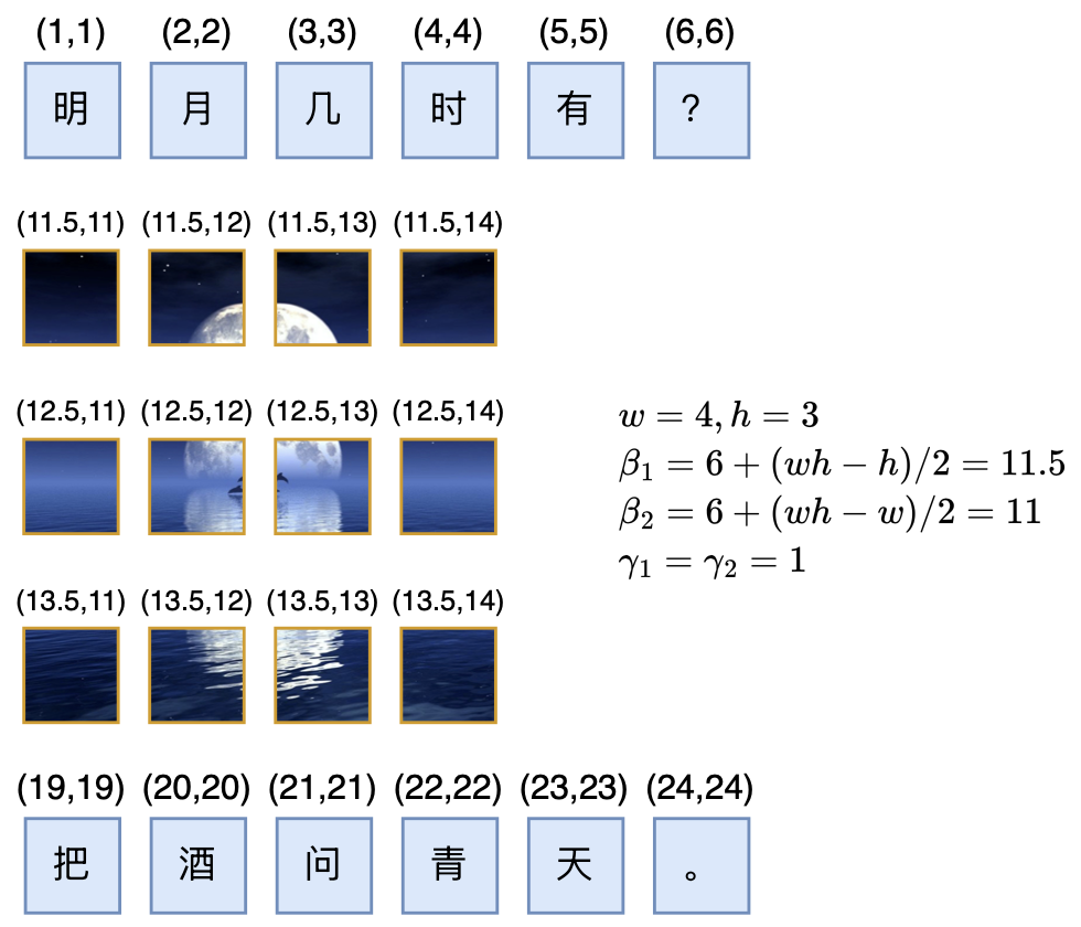
If the input is a single image with w \times h patches, its position coordinates are naturally the coordinates of the patches themselves, namely: \left[\begin{matrix} (1,1) & (1,2) & \cdots & (1, w) \\ (2,1) & (2,2) & \cdots & (2, w) \\ \vdots & \vdots & \ddots & \vdots \\ (h,1) & (h,2) & \cdots & (h, w) \\ \end{matrix}\right]\label{eq:rope2d} What we show here are absolute positions, but the actual effect is relative positioning. A characteristic of relative positioning is that it is independent of position bias, so we can add (\beta_1, \beta_2) to every coordinate without changing the effect. Secondly, we can multiply every coordinate by (\gamma_1, \gamma_2), allowing us to adjust the interval between adjacent positions as needed. Combining these two points, we get the generalized 2D positions for the image as: \left[\begin{matrix} (\beta_1 + \gamma_1,\beta_2 + \gamma_2) & (\beta_1 + \gamma_1,\beta_2 + 2\gamma_2) & \cdots & (\beta_1 + \gamma_1,\beta_2 + w\gamma_2) \\[8pt] (\beta_1 + 2\gamma_1,\beta_2 + \gamma_2) & (\beta_1 + 2\gamma_1,\beta_2 + 2\gamma_2) & \cdots & (\beta_1 + 2\gamma_1,\beta_2 + w\gamma_2) \\[8pt] \vdots & \vdots & \ddots & \vdots \\[8pt] (\beta_1 + h\gamma_1,\beta_2 + \gamma_2) & (\beta_1 + h\gamma_1,\beta_2 + 2\gamma_2) & \cdots & (\beta_1 + h\gamma_1,\beta_2 + w\gamma_2) \end{matrix}\right] Now we consider how to choose \beta_1, \beta_2, \gamma_1, \gamma_2 when an image is sandwiched between two segments of text.
First, we assume a certain equivalence between text tokens and patches: after reasonable Patchify, the status of each patch is equivalent to a token (An Image is Worth xxx Tokens). This means that for the two text segments, the image is equivalent to a sentence of wh tokens. So, if the last token of the left text segment is at position (L, L), then the first token of the right text segment is at position (L + wh + 1, L + wh + 1).
Next, we need to introduce symmetry. Specifically, the position of the first patch of the image is (\beta_1 + \gamma_1, \beta_2 + \gamma_2), and the position of the last patch is (\beta_1 + h\gamma_1, \beta_2 + w\gamma_2). We believe that the position difference between the [first patch of the image] and the [last token of the left text] should equal the position difference between the [first token of the right text] and the [last patch of the image], i.e.: \begin{pmatrix}\beta_1 + \gamma_1 \\ \beta_2 + \gamma_2\end{pmatrix} - \begin{pmatrix}L \\ L\end{pmatrix} = \begin{pmatrix}L+wh+1 \\ L+wh+1\end{pmatrix} - \begin{pmatrix}\beta_1 + h\gamma_1 \\ \beta_2 + w\gamma_2\end{pmatrix}\label{eq:beta-gamma} There are four unknowns \beta_1, \beta_2, \gamma_1, \gamma_2 here, but only two equations, so there are infinitely many solutions. We can simply set \gamma_1 = \gamma_2 = 1, and then solve for: \beta_1 = L + \frac{1}{2}(wh - h),\quad \beta_2 = L + \frac{1}{2}(wh - w) We can temporarily call this scheme RoPE-Tie-v2 or RoPE-TV (RoPE for Text and Vision).
Analysis of Pros and Cons
According to this result, when an image of w \times h patches follows a sentence, we only need to calculate (\beta_1, \beta_2) as described above and add them to the conventional 2D RoPE [eq:rope2d] to obtain the position coordinates for the image part, as shown in the figure below:
As a comparison, the position coordinates of the old RoPE-Tie proposed in “Path to Transformer Upgrade: 17. Simple Reflections on Multimodal Position Encoding” are shown in the figure below:
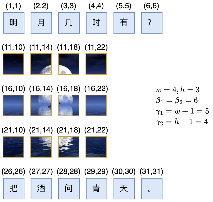
In fact, the starting point of RoPE-Tie also included compatibility and symmetry, but it did not strictly follow equivalence. Furthermore, RoPE-Tie defaulted to \beta_1 = \beta_2 = L and did not restrict w \times h patches to be equivalent to wh tokens, eventually leading to a set of integer solutions (if integer solutions are not required, equivalence can also be satisfied): \gamma_1 = w+1,\quad\gamma_2=h+1 From today’s perspective, the default settings of RoPE-Tie are not very ideal. Therefore, this article re-selects \gamma_1 = \gamma_2 = 1, ensures equivalence, and then derives \beta_1, \beta_2.
What are the benefits of the new scheme? First, in RoPE-Tie, the relative positions within the image depend on its size, whereas in the new scheme, the patch intervals are fixed at (0, 1) and (1, 0). This makes the scale of patches more consistent. For example, for a 128 \times 128 image and its upper half (a 128 \times 64 sub-image), because the heights are different, the horizontal position intervals in RoPE-Tie would be different. This means that two patches with the same position and meaning would have inconsistent distances (scales) after adding RoPE-Tie, which seems unreasonable. The new scheme does not have this problem.
Secondly, in RoPE-Tie, the interval between the image and the surrounding text is the same as the interval between patches within the image (\gamma_1, \gamma_2). In the new scheme, a relatively large interval \frac{1}{2}(wh - h, wh - w) appears between text and image, and between image and text, while the intervals within the text and within the image are fixed and uniform. Intuitively, this large positional jump between different modalities can better achieve “modality isolation,” allowing a single model to better process single-modality content while retaining multimodal interaction. This is similar to our usual practice of adding [IMG] and [/IMG] special tokens to mark the image.
The 3D Dilemma
In the RoPE-Tie article, position encoding for “text-video” mixed modalities was not discussed. In this section, we will complete that discussion.
Intuitively, there are two ways to handle video input. The first way is to simply treat the video as multiple images (adding [VIDEO] and [/VIDEO] markers if necessary). This way, we don’t need to propose a new position encoding for video and can just use the results of the “text-image” mixed position encoding. However, this loses the alignment relationship between different frames of the same video. For example, the “1st patch of the 1st frame” should have a similar proximity relationship to the “1st patch of the 2nd frame” as it does to the “2nd patch of the 1st frame,” but flattening it into multiple images fails to reflect this.
The second way is to extend the “text-image” results in parallel to “text-video.” For a video of w \times h \times t (screen size w \times h, total t frames), its position coordinates are 3D (x, y, z). Based on the same compatibility, equivalence, and symmetry, we can extend equation [eq:beta-gamma] to: \begin{pmatrix}\beta_1 + \gamma_1 \\ \beta_2 + \gamma_2 \\ \beta_3 + \gamma_3\end{pmatrix} - \begin{pmatrix}L \\ L \\ L\end{pmatrix} = \begin{pmatrix}L+wht+1 \\ L+wht+1 \\ L+wht+1\end{pmatrix} - \begin{pmatrix}\beta_1 + h\gamma_1 \\ \beta_2 + w\gamma_2 \\ \beta_3 + t\gamma_3\end{pmatrix} If we still set \gamma_1 = \gamma_2 = \gamma_3 = 1, we get: \beta_1 = L + \frac{1}{2}(wht - h),\quad \beta_2 = L + \frac{1}{2}(wht - w),\quad \beta_3 = L + \frac{1}{2}(wht - t)
This approach fully preserves the 3D nature of video positions and looks more elegant, but the author believes it still has some shortcomings.
This shortcoming stems from the author’s different understanding of the time dimension of video: the three dimensions of video are actually “2 spatial dimensions + 1 time dimension,” which is different from the “3 spatial dimensions” of the real 3D world. In the author’s view, the time dimension of video is not equal to the two spatial dimensions. The time dimension is more like the left-to-right writing direction of text. Therefore, the perfect multimodal LLM in the author’s imagination should be able to continue a video autoregressively, just as a text LLM continues text, theoretically capable of infinite video generation until an [EOS] token appears.
We just mentioned two “text-video” mixed encoding schemes. The first one treats it as multiple images, and this scheme allows for infinite autoregressive video generation. However, the second, seemingly more perfect scheme does not, because its \beta_1, \beta_2, \beta_3 depend on t. This means we need to know in advance how many frames of video to generate. In other words, the second scheme is not unusable for autoregressive video generation, but it requires pre-determining the number of frames, which in the author’s view does not fit the ideal characteristics of the time dimension (time should be able to advance forward without constraints).
Some readers might ask: why don’t we mind \beta_1, \beta_2 depending on w, h for images? That is, why don’t we mind knowing the image size in advance for image generation? This is because images have two directions. Even if we generate an image autoregressively, we must know the size of at least one direction to tell the model when to “wrap” to generate a complete 2D image. Since the two spatial dimensions of an image are equal, it’s better to know both than just one, so we can accept pre-determining the image size.
Furthermore, we can use the “AR+Diffusion” model introduced in “Building a Car Behind Closed Doors”: A Brief Discussion on Multimodal Ideas (Part 1): Lossless Input”. In this case, the image generation part is Diffusion, which must know the target image size in advance.
Related Work
Recently, Alibaba open-sourced a multimodal model named “Qwen2-VL.” The introduction mentioned that they proposed a Multimodal Rotary Position Encoding (M-ROPE), which piqued the author’s interest. After reading the source code (link), I found that M-RoPE actually follows the compatibility idea of RoPE-Tie but does not preserve symmetry and equivalence.
Using the notation of this article, M-RoPE actually sets \beta_1 = \beta_2 = \beta_3 = L, \gamma_1 = \gamma_2 = \gamma_3 (for “text-video” mixed modality), and then the position of the first token of the text following the video is simply the maximum video coordinate plus 1. This way, if video is still generated autoregressively, there is indeed no need to pre-determine the number of frames, but symmetry and equivalence are sacrificed.
How important are symmetry and equivalence? The author does not know the answer; it requires sufficient experimentation to verify. But if it’s just brainstorming, the author guesses it might affect performance in extreme cases. For example, in M-RoPE, for a video with a very small screen but a very long duration, its spatial position coordinates would be continuous relative to the left text but would jump abruptly relative to the right text. Intuitively, this might make the interaction between text and vision less friendly.
Another example: for a video where w=h=t=n, it intuitively is equivalent to n^3 tokens. However, according to M-RoPE rules, if such a video is sandwiched between two text segments, it is only equivalent to being sandwiched by n text tokens. In other words, n^3 tokens are placed within a relative distance of size n. Could this lead to excessive information density and increase the difficulty of model understanding?
Of course, for Decoder-only LLMs where even NoPE (No Position Encoding) might work, these concerns might just be the author overthinking.
Summary
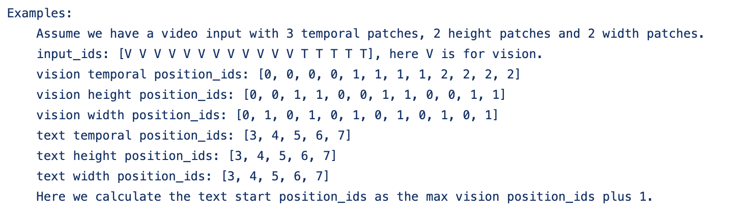
This article shares the author’s subsequent reflections on multimodal position encoding, proposing three principles for constructing multimodal position encoding: compatibility, equivalence, and symmetry. It improves upon the previously proposed RoPE-Tie and finally discusses the design and difficulties of position encoding for “text-video” mixed modalities, as well as the connection between Qwen2-VL’s M-RoPE and RoPE-Tie.
Original Address: https://kexue.fm/archives/10352
For more details on reprinting, please refer to: Scientific Space FAQ