When reviewing mainstream image diffusion model works, we notice a distinct characteristic: most current work on high-resolution image generation (hereinafter referred to as "large image generation") is conducted by transforming into a Latent space via an Encoder (i.e., LDM, Latent Diffusion Model). Diffusion models trained directly in the original Pixel space mostly have resolutions not exceeding 64 \times 64. Coincidentally, the Latent size after LDM transformation via an AutoEncoder usually does not exceed 64 \times 64 either. This naturally leads to a series of questions: Does the diffusion model have inherent difficulties with high-resolution generation? Can high-resolution images be generated directly in Pixel space?
The paper "Simple diffusion: End-to-end diffusion for high resolution images" attempts to answer this question. It analyzes the difficulties of large image generation through the concept of "Signal-to-Noise Ratio" (SNR) and uses this to optimize the noise schedule. Simultaneously, it proposes techniques such as scaling up the architecture only on the lowest resolution features and using multi-scale Loss to ensure training efficiency and effectiveness. These modifications allowed the original paper to successfully train image diffusion models with resolutions as high as 1024 \times 1024 in Pixel space.
LDM Review
Before diving into the main topic, let’s think in reverse: Why has LDM successfully become the mainstream approach for diffusion models? I believe there are two main reasons:
1. Whether in application or academia, the primary reason for using LDM is likely efficiency: current mainstream works directly reuse the pre-trained AutoEncoder open-sourced by the LDM paper. Its Encoder transforms a 512 \times 512 image into a 64 \times 64 Latent. This means that by using computational power and time equivalent to the 64 \times 64 resolution level, one can generate 512 \times 512 images. This efficiency is obviously very attractive.
2. LDM aligns well with the FID metric, making it appear lossless in terms of performance: FID stands for "Fréchet Inception Distance," where "Inception" refers to using the InceptionV3 model pre-trained on ImageNet as an Encoder to encode images, and then calculating the \mathcal{W} distance assuming the encoded features follow a Gaussian distribution. Since LDM also uses an Encoder, and although the two Encoders are not identical, they share certain commonalities, LDM performs as if it were almost lossless in terms of FID.
We can expand on this slightly. The AutoEncoder in LDM combines many elements during the training phase—its reconstruction Loss is not just the conventional MAE or MSE, but also includes Adversarial Loss and Perceptual Loss. The Adversarial Loss is used to ensure the clarity of the reconstruction results, while the Perceptual Loss is used to ensure the similarity of the semantics and style of the reconstruction. Perceptual Loss is very similar to FID; both are similarity metrics calculated using features from ImageNet models, except it uses VGG-16 instead of InceptionV3. Due to the similarity of the training tasks, one can guess that their features share many commonalities. Therefore, the inclusion of Perceptual Loss disguisedly ensures that the FID loss is minimized.
Furthermore, the LDM Encoder performs dimensionality reduction on the original image. For example, if the original image size is 512 \times 512 \times 3, direct patchification results in 64 \times 64 \times 192, but the features from the LDM Encoder are 64 \times 64 \times 4, reduced to 1/48. Meanwhile, to further reduce the variance of the encoded features and prevent the model from "rote memorization," LDM also adds corresponding regularization terms to the Encoder features, such as the KL divergence term of VAE or the VQ regularization of VQ-VAE. The design of dimensionality reduction and regularization compresses the diversity of features and improves their generalization ability, but it also increases the difficulty of reconstruction, ultimately leading to lossy reconstruction results.
At this point, the reason for LDM’s success becomes "crystal clear": the combination of "dimensionality reduction + regularization" reduces the information content of the Latent, thereby reducing the difficulty of learning the diffusion model in Latent space. Meanwhile, the existence of Perceptual Loss ensures that although the reconstruction is lossy, the FID is almost lossless (theoretically, it would be even better if the Perceptual Loss Encoder used InceptionV3 like FID). Consequently, for the FID metric, LDM is almost a free lunch, which is why both academia and industry are happy to continue using it.
Signal-to-Noise Ratio
Despite LDM being simple and efficient, it is ultimately lossy. Its Latent can only maintain macro-level semantics, and local details may be severely missing. In a previous article, "Building Cars Behind Closed Doors" - Thoughts on Multimodal Approaches (1): Lossless Input, I expressed the view that when used as input, the best representation of an image is the original Pixel array. Based on this view, I have recently been paying more attention to diffusion models trained directly in Pixel space.
However, when applying the configuration of a low-resolution (e.g., 64 \times 64) image diffusion model directly to high-resolution (e.g., 512 \times 512) large image generation, problems such as excessive computational consumption and slow convergence arise. Moreover, the results are not as good as LDM (at least according to the FID metric). Simple diffusion analyzes these problems one by one and proposes corresponding solutions. Among them, I find the use of the "Signal-to-Noise Ratio (SNR)" concept to analyze the low learning efficiency of high-resolution diffusion models to be the most brilliant.
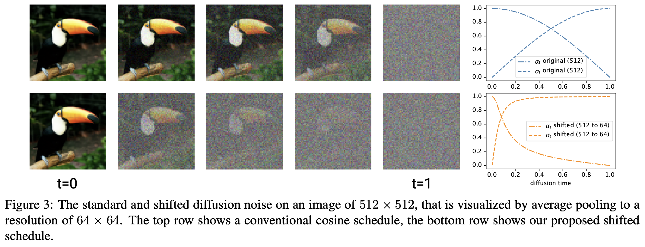
Specifically, Simple diffusion observed that if we add noise of a certain variance to a high-resolution image, its signal-to-noise ratio is actually higher compared to a low-resolution image with the same noise variance. Figure 3 of the original paper demonstrates this very intuitively, as shown below. The first row of images consists of 512 \times 512 images with specific noise variance added, then downsampled (Average Pooling) to 64 \times 64. The second row consists of 64 \times 64 images with the same noise variance added directly. It is clear that the images in the first row are clearer, meaning the relative signal-to-noise ratio is higher.
The so-called "Signal-to-Noise Ratio," as the name suggests, is the "ratio of the intensity of the signal to the noise." A higher SNR (meaning a lower proportion of noise) means denoising is easier. In other words, during the training phase, the Denoiser mostly faces simple samples. However, in reality, the difficulty of large image generation is clearly higher. That is to say, our goal is a more difficult model, but we provide simpler samples, which leads to low learning efficiency.
Aligning Downwards
We can also describe this mathematically. Using the notation of this series, the operation of constructing \boldsymbol{x}_t through noise addition can be expressed as: \boldsymbol{x}_t = \bar{\alpha}_t \boldsymbol{x}_0 + \bar{\beta}_t \boldsymbol{\varepsilon},\quad \boldsymbol{\varepsilon}\sim\mathcal{N}(\boldsymbol{0},\boldsymbol{I}) where \bar{\alpha}_t, \bar{\beta}_t are called the noise schedule, satisfying \bar{\alpha}_0=\bar{\beta}_T=1, \bar{\alpha}_T=\bar{\beta}_0=0. Furthermore, they generally have additional constraints; for example, in DDPM, it is usually \bar{\alpha}_t^2 + \bar{\beta}_t^2=1. This article will follow this constraint.
For a random variable, the signal-to-noise ratio is the ratio of the square of the mean to the variance. Given \boldsymbol{x}_0, the mean of \boldsymbol{x}_t is clearly \bar{\alpha}_t \mathbb{E}[\boldsymbol{x}_0], and the variance is \bar{\beta}_t^2. Thus, the signal-to-noise ratio is \frac{\bar{\alpha}_t^2}{\bar{\beta}_t^2}\mathbb{E}[\boldsymbol{x}_0]^2. Since we always discuss this given \boldsymbol{x}_0, we can simply say the signal-to-noise ratio is: SNR(t) = \frac{\bar{\alpha}_t^2}{\bar{\beta}_t^2}
When we apply s \times s Average Pooling to \boldsymbol{x}_t, each s \times s patch is transformed into a scalar by taking the average: \frac{1}{s^2}\sum_{i=1}^s \sum_{j=1}^s\boldsymbol{x}_t^{(i,j)} = \bar{\alpha}_t\left(\frac{1}{s^2}\sum_{i=1}^s \sum_{j=1}^s \boldsymbol{x}_0^{(i,j)}\right) + \bar{\beta}_t\left(\frac{1}{s^2}\sum_{i=1}^s \sum_{j=1}^s \boldsymbol{\varepsilon}^{(i,j)}\right) ,\quad \boldsymbol{\varepsilon}^{(i,j)}\sim\mathcal{N}(0, 1) Average Pooling does not change the mean but reduces the variance, thereby increasing the signal-to-noise ratio. This is because the additivity of the normal distribution implies: \frac{1}{s^2}\sum_{i=1}^s \sum_{j=1}^s \boldsymbol{\varepsilon}^{(i,j)}\sim\mathcal{N}(0, 1/s^2) So, under the same noise schedule, if we align a high-resolution image to a low-resolution one via Average Pooling, we find that the signal-to-noise ratio is higher, specifically s^2 times the original: SNR^{w\times h\to w/s\times h/s}(t) = SNR^{w/s\times h/s}(t) \times s^2 Thinking in reverse, if we already have a noise schedule \bar{\alpha}_t^{w/s\times h/s}, \bar{\beta}_t^{w/s\times h/s} tuned for low-resolution images, then when we want to scale up to a higher resolution, we should adjust the noise schedule to \bar{\alpha}_t^{w\times h}, \bar{\beta}_t^{w\times h} such that after downsampling to low resolution, its signal-to-noise ratio aligns with the already tuned low-resolution noise schedule. This way, we can "inherit" the learning efficiency of the low-resolution diffusion model to the greatest extent: \frac{(\bar{\alpha}_t^{w\times h})^2}{(\bar{\beta}_t^{w\times h})^2} \times s^2 = \frac{(\bar{\alpha}_t^{w/s\times h/s})^2}{(\bar{\beta}_t^{w/s\times h/s})^2} If we add the constraint \bar{\alpha}_t^2 + \bar{\beta}_t^2=1, then \bar{\alpha}_t^{w\times h}, \bar{\beta}_t^{w\times h} can be uniquely solved from \bar{\alpha}_t^{w/s\times h/s}, \bar{\beta}_t^{w/s\times h/s}. This solves the noise schedule setting problem for high-resolution diffusion.
Architecture Scaling
To perform high-resolution diffusion generation well, in addition to adjusting the noise schedule, we also need to scale up the architecture. As mentioned earlier, large image generation is a more difficult problem, so it naturally requires a more heavyweight architecture.
Diffusion models commonly use U-Net or U-Vit. Both gradually downsample and then gradually upsample. For example, with a 512 \times 512 input, one block of computation is performed, then it is downsampled to 256 \times 256, followed by another block of computation, then downsampled to 128 \times 128, and so on, down to a minimum resolution of 16 \times 16. Then the process is repeated but with upsampling until the resolution returns to 512 \times 512. By default, we distribute parameters equally across each block. However, this causes the computational load of blocks near the input and output to increase sharply because their input sizes are very large, making model training inefficient or even infeasible.
Simple diffusion proposes two solutions. First, it suggests downsampling immediately after the first layer (not the first block, as each block has multiple layers) and considers downsampling directly to 128 \times 128 or even 64 \times 64 in one step. Finally, for the output, it only upsamples from 64 \times 64 or 128 \times 128 back to 512 \times 512 just before the last layer. This way, the resolution processed by most blocks in the model is reduced, thereby reducing the overall computational load. Second, it proposes placing the scaled-up layers of the model after the lowest resolution (i.e., 16 \times 16) rather than spreading them across blocks of every resolution. That is, the newly added layers all process 16 \times 16 inputs, and Dropout is also only added to the low-resolution layers. In this way, the computational pressure brought by the increase in resolution is significantly reduced.
Furthermore, to further stabilize training, the paper proposes a "multi-scale Loss" training objective. By default, the Loss of a diffusion model is equivalent to the MSE loss: \mathcal{L}=\frac{1}{wh}\Vert \boldsymbol{\varepsilon} - \boldsymbol{\epsilon}_{\boldsymbol{\theta}}(\bar{\alpha}_t \boldsymbol{x}_0 + \bar{\beta}_t \boldsymbol{\varepsilon}, t)\Vert^2 Simple diffusion generalizes this to: \mathcal{L}_{s\times s} = \frac{1}{(w/s)(h/s)}\big\Vert \mathcal{D}_{w/s\times h/s}[\boldsymbol{\varepsilon}] - \mathcal{D}_{w/s\times h/s}[\boldsymbol{\epsilon}_{\boldsymbol{\theta}}(\bar{\alpha}_t \boldsymbol{x}_0 + \bar{\beta}_t \boldsymbol{\varepsilon}, t)]\big\Vert^2 where \mathcal{D}_{w/s\times h/s}[\cdot] is a downsampling operator that transforms the input to w/s \times h/s via Average Pooling. The original paper takes the average of Losses corresponding to multiple s values as the final training objective. The goal of this multi-scale Loss is also clear: like adjusting the noise schedule through SNR alignment, it ensures that the trained high-resolution diffusion model is at least as good as a directly trained low-resolution model.
As for the experimental part, readers can refer to the original paper. The maximum resolution experimented with in Simple diffusion is 1024 \times 1024 (mentioned in the appendix), and the results are acceptable. Comparative experiments show that the techniques proposed above all provide improvements. Ultimately, the diffusion model trained directly in Pixel space achieved competitive results compared to LDM.
Summary
In this article, we introduced Simple diffusion, a work that explores how to train image diffusion models end-to-end directly in Pixel space. It utilizes the concept of Signal-to-Noise Ratio to explain the low training efficiency of high-resolution diffusion models, uses this to adjust a new noise schedule, and explores how to scale up the model architecture while saving computational costs as much as possible.
Reprinting: Please include the original address of this article: https://kexue.fm/archives/10047
More details: For more detailed reprinting matters, please refer to: "Scientific Space FAQ"