Looking at the Scale Operation of Attention from the Perspective of Gradient Maximization

Existing Results

In "A Brief Talk on Initialization, Parameterization, and Normalization of Transformer", we previously derived the standard scale factor \frac{1}{\sqrt{d}}. The derivation logic was simple: assuming that in the initial stage, \boldsymbol{q}, \boldsymbol{k} \in \mathbb{R}^d are sampled from a distribution with "mean 0 and variance 1," we can calculate: \begin{equation} \mathbb{V}ar[\boldsymbol{q}\cdot\boldsymbol{k}] = d \end{equation} Thus, we divide \boldsymbol{q}\cdot\boldsymbol{k} by \sqrt{d} to make the variance of the Attention Score equal to 1. In other words, the previous derivation was purely based on the belief that "mean 0 and variance 1" is better. However, it did not explain why making the variance of the Attention Score 1 is optimal, nor did it evaluate whether \frac{1}{\sqrt{d}} truly solves the vanishing gradient problem.

Of course, based on existing experiments, \frac{1}{\sqrt{d}} alleviates this problem to some extent. But since these are experimental results, we still hope to understand theoretically how much "to some extent" actually is.

Calculating Gradients

Since gradients are involved, the best approach is to calculate the gradient and define an optimization objective. Let p_i = e^{\alpha s_i}/Z, where i \in \{1,2,...,n\} and Z=\sum_i e^{\alpha s_i} is the normalization factor. We can directly calculate: \begin{equation} \frac{\partial p_i}{\partial s_j} = \left\{\begin{aligned} \alpha(p_i - p_i^2),&\quad i=j\\ -\alpha p_i p_j,&\quad i\neq j \end{aligned}\right. \end{equation} Or it can be written concisely as \partial p_i/\partial s_j = \alpha(p_i\delta_{i,j} - p_i p_j). Obviously, when \alpha \to 0, the gradient is 0; when \alpha \to \infty, only one p_i is 1 and the rest are 0 (assuming there is a unique maximum among s_i), and the gradient is also 0.

To facilitate optimization, we should choose \alpha such that the gradient is maximized. To this end, we use the L1 norm as a measure of the gradient magnitude: \begin{equation} \frac{1}{2}\left\Vert\frac{\partial p}{\partial s}\right\Vert_1 = \frac{1}{2}\sum_{i,j}\left|\frac{\partial p_i}{\partial s_j}\right| = \frac{1}{2}\sum_i \alpha(p_i - p_i^2) + \frac{1}{2}\sum_{i\neq j} \alpha p_i p_j = \alpha\left(1 - \sum_i p_i^2\right) \label{eq:target} \end{equation} It is not hard to guess that the fundamental reason for choosing L1 over others is that the calculation result for the L1 norm is sufficiently simple. It is worth noting that \sum_i p_i^2 appears here; it is essentially the "Rényi entropy" introduced in "How to Measure the Sparsity of Data?". Similar to information entropy, it is also a measure of uncertainty.

With the optimization objective in hand, we can proceed to maximize it. Note that the definition of p_i also contains \alpha, so this is a complex non-linear objective regarding \alpha. While an analytical solution seems impossible, we can find approximate solutions for some specific cases.

Normal Distribution

First, we can build upon the previous results. When we make the mean of the Attention Score 0 and the variance 1 by dividing by \sqrt{d}, we can approximately assume s_i \sim \mathcal{N}(0,1) and then solve for the optimal \alpha. If \alpha=1, it means the original \frac{1}{\sqrt{d}} is the optimal scale ratio; otherwise, \frac{\alpha}{\sqrt{d}} is the best scale ratio.

We use expectation to estimate the sum: \begin{equation} \sum_i p_i^2 = \frac{\sum_i e^{2\alpha s_i}}{\left(\sum_i e^{\alpha s_i}\right)^2} = \frac{\frac{1}{n}\sum_i e^{2\alpha s_i}}{n\left(\frac{1}{n}\sum_i e^{\alpha s_i}\right)^2} \approx \frac{\mathbb{E}_s[e^{2\alpha s}]}{n\left(\mathbb{E}_s[e^{\alpha s}]\right)^2} \label{eq:approx} \end{equation} For s following a standard normal distribution, we have: \begin{equation} \mathbb{E}_s[e^{\alpha s}] = \int \frac{1}{\sqrt{2\pi}}e^{-s^2/2}e^{\alpha s} ds = e^{\alpha^2 / 2} \label{eq:normal} \end{equation} Substituting this into the above equation and then into Equation [eq:target], we get: \begin{equation} \alpha\left(1 - \sum_i p_i^2\right) \approx \alpha\left(1 - \frac{e^{\alpha^2}}{n}\right) \end{equation} Although the final approximation is simplified, it is still not easy to find the maximum value analytically. However, we can iterate through some values of n and numerically solve for the \alpha^* that yields the maximum value. This allows us to see the relationship between \alpha^* and n. The reference Mathematica code is as follows:

(* Define function *)
f[a_, n_] := a*(1 - Exp[a^2]/n)
(* Find the point a corresponding to the maximum of the function *)
FindArg[n_] := 
 Module[{a}, a = a /. Last@NMaximize[{f[a, n], a > 0}, a][[2]]; a]
(* Given range of n *)
nRange = 40*Range[1, 500];
(* Calculate a for each n *)
args = FindArg /@ nRange;
(* Plot the relationship between a and n *)
ListLinePlot[{args, 0.84*Log[nRange]^0.5}, 
 DataRange -> {40, 20000}, AxesLabel -> {"n", "a"}, 
 PlotLegends -> {Row[{"a", Superscript["", "*"]}], 
   TraditionalForm[HoldForm[0.84*Sqrt[Log[n]]]]}]

Through fitting, the author found that within a certain range, the optimal point \alpha^* and n roughly satisfy the relationship \alpha \approx 0.84\sqrt{\log n}. The corresponding approximate function is plotted together below:

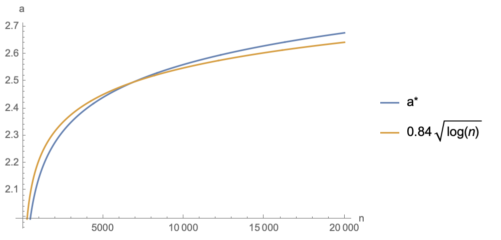
As can be seen, over a fairly large range, the optimal value of \alpha^* is between 2 and 3. Therefore, as a compromise, choosing \frac{2.5}{\sqrt{d}} as the Attention scale factor is theoretically more conducive to optimization.

Cosine Distribution

Now let’s consider another less common example: when we apply l_2 normalization to both \boldsymbol{q} and \boldsymbol{k} to make them unit vectors, their dot product becomes the cosine of the angle between them. That is, s_i approximately follows the distribution of the cosine of the angle between two random vectors in a d-dimensional space. This distribution might be unfamiliar to some readers, but we explored it in "Angle Distribution of Two Random Vectors in n-dimensional Space". Its probability density has the form: \begin{equation} p(s) \propto (1-s^2)^{(d-3)/2} \end{equation}

It doesn’t look complicated, but in fact, this form is much harder to handle than the normal distribution, mainly because \mathbb{E}_s[e^{\alpha s}] cannot be expressed in elementary functions like in Equation [eq:normal]. However, this is not a problem for numerical solving in Mathematica. Following the same logic as the previous section, the approximation in Equation [eq:approx] still applies. We first solve for the maximum value numerically and then fit it. The results are as follows (in the figure d=128, and \alpha^* is related to d):

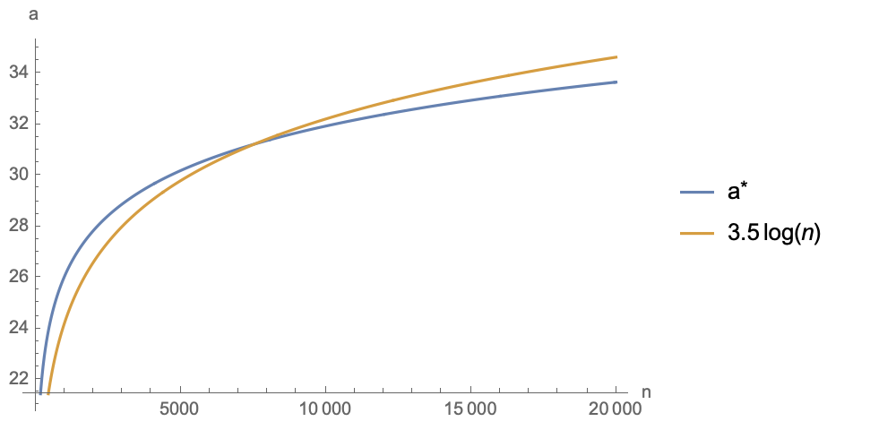
It can be seen that \alpha^* fits well with 3.5\log n (if d changes, the coefficient 3.5 will change). Within a fairly large range, \alpha^* is between 25 and 35. Therefore, if cosine similarity is used as the Attention Score, it needs to be multiplied by a scale between 25 and 35 to make the model trainable. This also explains why when using cosine values to construct Softmax distributions (such as in AM-Softmax, SimCSE, etc.), we need to multiply the cosine by a scale of around 30; otherwise, it is very difficult to train the model.

For different d and n, readers can modify the following code to calculate the optimal \alpha:

(* Define function *)
h[a_] := 
 Integrate[Exp[a*s]*(1 - s^2)^((d - 3)/2), {s, -1, 1}, 
  Assumptions -> {d > 10}]
g[a_] = h[a]/h[0] // FullSimplify;
f[a_, n_] := a (1 - g[2*a]/g[a]^2/n) /. {d -> 128}
(* Find the point a corresponding to the maximum of the function *)
FindArg[n_] := 
 Module[{a}, a = a /. Last@NMaximize[{f[a, n], a > 0}, a][[2]]; a]
(* Given range of n *)
nRange = 40*Range[1, 500];
(* Calculate a for each n *)
args = FindArg /@ nRange;
(* Plot the relationship between a and n *)
ListLinePlot[{args, 3.5*Log[nRange]}, 
 DataRange -> {40, 20000}, AxesLabel -> {"n", "a"}, 
 PlotLegends -> {Row[{"a", Superscript["", "*"]}], 
   TraditionalForm[HoldForm[3.5*Log[n]]]}]

Related Thoughts

The title and results of this article, especially the result that \alpha is approximately proportional to \log n in the cosine distribution, easily remind us of another article discussing Attention Scale: "Looking at the Scale Operation of Attention from the Perspective of Entropy Invariance". In fact, a connection between the two articles does exist. The optimization objective [eq:target] in this article involves "Rényi entropy," while the entropy in "entropy invariance" refers to Shannon information entropy. The properties of the two are largely consistent. Maximizing Equation [eq:target] puts it into a "slowly changing" region, which means that the change of "Rényi entropy" with respect to n is very slow, implying that the change of information entropy with respect to n is also very slow. This is roughly equivalent to entropy invariance.

Furthermore, for bidirectional Attention (Encoder), assuming the training sample lengths are the same, n is a constant. We can calculate the corresponding optimal \alpha based on n and fix it in the model. However, for unidirectional Attention (Decoder), the n for each token is actually different (position ID plus 1). Therefore, theoretically, it is impossible to maximize Equation [eq:target] for all tokens. But since \alpha^* changes slowly with respect to n, taking a reasonable value is sufficient. For example, one could take n=L_{\max} / 2, which would be gradient-friendly for most tokens.

Summary

This article explores the selection of the Attention scale factor from the perspective of gradients. It is well known that the "standard answer" for this scale factor is \frac{1}{\sqrt{d}}, but its derivation does not discuss its optimality. Therefore, the author defined an optimization objective for the Softmax gradient and explored the optimal value of the scale factor by maximizing this objective. The relevant results can be used to improve the scale factor of Attention and to explain the temperature parameter in contrastive learning using cosine similarity.

Original URL: https://kexue.fm/archives/9812