Google's New Work Attempts to ``Resurrect'' RNN: Can RNN Shine Again?

Linearization

The RNN proposed in the article is called LRU (Linear Recurrent Unit). It is a minimalist linear RNN that can be both parallelized and serialized, offering efficiency in both training and inference. LRU shares many similarities with works like SSM (Structured State Model) and RWKV. In fact, the starting point for LRU was the discovery that SSM performs well on the LRA benchmark, leading the authors to find a way to make native RNNs perform well on LRA too; the result is LRU. Unfortunately, the original paper only conducted experiments on LRA (Long Range Arena, a benchmark for testing long-range dependency capabilities). At the end of this article, I will supplement some of my own experimental results on language models.

The original paper introduces LRU starting from SSM and spends considerable space describing the connection between the two. In this article, we will skip those descriptions and derive LRU directly as an independent RNN model. We know that the simplest RNN can be written as: \begin{equation} x_t = f(Ax_{t-1} + u_t) \end{equation} where x_t, u_t \in \mathbb{R}^d, A \in \mathbb{R}^{d \times d}, and f is the activation function. Generally, there are projection matrices before u_t and after x_t, but here we focus on the recurrence itself, so we won’t write them explicitly.

In traditional understanding, activation functions are non-linear, with common choices being \text{sigmoid}, \tanh, \text{relu}, etc. In particular, some work has shown that a single-layer RNN with \text{sigmoid} or \tanh activation is Turing complete, which reinforces the belief in the necessity of non-linear activations. However, in deep learning, experiment is the sole criterion for testing truth. The authors found that if the Self-Attention in a Transformer is replaced by an RNN, a linear RNN actually performs best:

This is a surprising piece of good news. It is “surprising” because it might overturn some readers’ perceptions regarding the model’s need for non-linearity. Of course, some readers might not be surprised, as works like MetaFormer have shown that thanks to the power of the FFN layer, the non-linearity of layers responsible for mixing tokens (like Self-Attention) can be very weak, or even replaced by a Pooling layer. As for the “good news,” it is because linear RNNs have parallel implementation algorithms, making their calculation speed much faster than non-linear RNNs.

Thus, the authors conducted a series of discussions centered around linear RNNs.

Diagonalization

By removing the activation function, the RNN simplifies to: \begin{equation} x_t = Ax_{t-1} + u_t\label{eq:lr} \end{equation} Iterating repeatedly yields: \begin{equation} \begin{aligned} x_0 &= u_0 \\ x_1 &= Au_0 + u_1 \\ x_2 &= A^2 u_0 + Au_1 + u_2 \\ &\vdots \\ x_t &= \sum_{k=0}^t A^{t-k}u_k \end{aligned} \label{eq:lr-e} \end{equation} As we can see, the main computational load is concentrated on the power operations of matrix A. At this point, it is natural to think of matrix diagonalization, which is an efficient method for calculating matrix powers. However, a general matrix may not be diagonalizable in the real field. What should we do? Let’s broaden our perspective: if it can’t be done in the real field, we go to the complex field! Almost all matrices can be diagonalized in the complex field, which means A can always be written as: \begin{equation} A = P\Lambda P^{-1} \quad \Rightarrow \quad A^n = P\Lambda^n P^{-1} \end{equation} where P, \Lambda \in \mathbb{C}^{d \times d}, and \Lambda is a diagonal matrix composed of eigenvalues. Substituting this into Equation [eq:lr-e], we get: \begin{equation} x_t = \sum_{k=0}^t P\Lambda^{t-k}P^{-1}u_k = P\left(\sum_{k=0}^t \Lambda^{t-k}(P^{-1}u_k)\right) \end{equation} As mentioned earlier, there are usually projection matrices before u_t and after x_t. As long as we stipulate that these two projection matrices are complex matrices, then theoretically P and P^{-1} can be merged into their projection operations. This means that if all operations are considered in the complex field, replacing the general matrix A in a linear RNN with a diagonal matrix \Lambda will not result in any loss of model capability! Therefore, we only need to consider the following minimalist RNN: \begin{equation} x_t = \Lambda x_{t-1} + u_t \quad \Rightarrow \quad x_t = \sum_{k=0}^t \Lambda^{t-k}u_k\label{eq:lr-x} \end{equation}

Parameterization

The advantage of a diagonal matrix is that all operations are element-wise, so the operations for each dimension can be fully parallelized. This also means that analyzing one dimension is equivalent to analyzing all dimensions; the model analysis only needs to be conducted in a one-dimensional space. Let \Lambda = \text{diag}(\lambda_1, \lambda_2, \dots, \lambda_d), where \lambda represents one of \lambda_1, \lambda_2, \dots, \lambda_d. Without loss of clarity, x_t and u_t are also used to represent the corresponding components of \lambda. Thus, Equation [eq:lr-x] simplifies to scalar operations: \begin{equation} x_t = \lambda x_{t-1} + u_t \quad \Rightarrow \quad x_t = \sum_{k=0}^t \lambda^{t-k}u_k\label{eq:lr-xx} \end{equation} Note that \lambda is a complex number, so we can set \lambda = re^{i\theta}, where r \geq 0 and \theta \in [0, 2\pi) are real numbers: \begin{equation} x_t = \sum_{k=0}^t r^{t-k}e^{i(t-k)\theta}u_k\label{eq:lr-e-r-theta} \end{equation} In the summation process, t-k is always non-negative, so r \leq 1. Otherwise, the weight of historical terms will gradually tend toward infinity, which contradicts intuition (intuitively, dependence on historical information should gradually weaken) and poses a risk of gradient explosion. On the other hand, if r \ll 1, there is a risk of gradient vanishing. This places two requirements on r: 1. Ensure r \in [0, 1]; 2. In the initialization phase, r should be as close to 1 as possible.

To this end, we first set r = e^{-\nu}. Then r \in [0, 1] requires \nu \geq 0. Thus, we further set \nu = e^{\nu^{\log}}, which makes \nu^{\log} \in \mathbb{R} and transforms the problem into unconstrained optimization. Here \nu^{\log} is just a notation for another variable, not representing any special operation. Since \nu is parameterized as e^{\nu^{\log}}, to maintain consistency, we also parameterize \theta as e^{\theta^{\log}}.

Readers might ask: there are many ways to constrain r \in [0, 1], why make it so complicated? Wouldn’t adding a sigmoid be simpler? First, after parameterizing r as e^{-\nu}, the power operation can be combined with \theta, i.e., r^k e^{ik\theta} = e^{k(-\nu + i\theta)}, which is better from both implementation and calculation perspectives. Second, since \nu \geq 0, the simplest smooth function that maps any real number to a non-negative number is likely the exponential function, hence \nu = e^{\nu^{\log}}. SSM uses \text{relu} activation, i.e., r = e^{-\max(\nu, 0)}, but this has a saturation zone which might be unfavorable for optimization.

Initialization

Next, consider the initialization problem. Returning to the original form [eq:lr], for a d \times d real matrix, the standard Glorot initialization is a normal or uniform distribution with mean 0 and variance 1/d (refer to “Understanding Model Parameter Initialization Strategies from a Geometric Perspective”). It can be shown theoretically or experimentally that the eigenvalues of such an initialized matrix are roughly uniformly distributed within the unit circle on the complex plane:

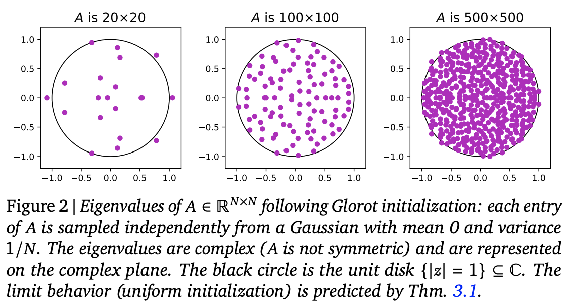
From this, we can think of the standard initialization for \Lambda as taking points uniformly within the unit circle on the complex plane. Converting from Cartesian to polar coordinates, we have dxdy = rdrd\theta = \frac{1}{2}d(r^2)d\theta. This tells us that to achieve uniform sampling within the unit circle, we only need \theta \sim U[0, 2\pi] and r^2 \sim U[0, 1].

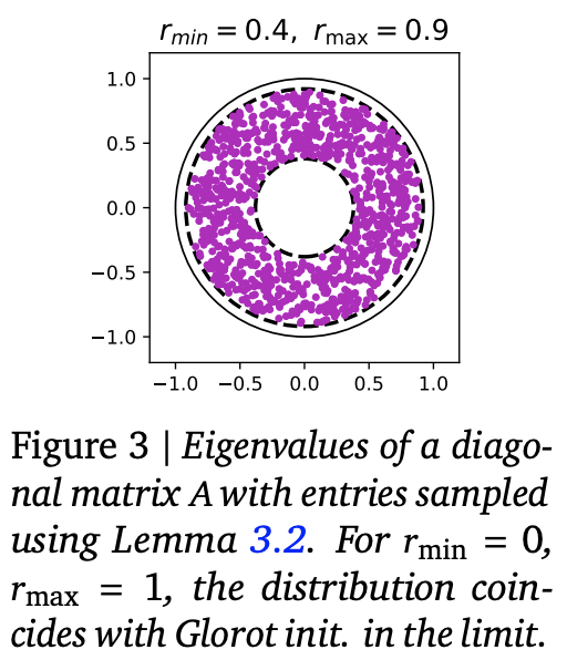
However, as we just said, to prevent gradient vanishing as much as possible, we should make r as close to 1 as possible during initialization. Therefore, the improved method is to sample uniformly within a ring where r \in [r_{\min}, r_{\max}]. The sampling method becomes \theta \sim U[0, 2\pi] and r^2 \sim U[r_{\min}^2, r_{\max}^2]. Experimental results in the original paper show that r_{\min}=0.9, r_{\max}=0.999 works well for most experiments.

There is a problem here: if r is initialized close to 1, and in the initial stage u_t is also close to i.i.d., then Equation [eq:lr-e-r-theta] is close to a sum of several terms with constant magnitude (rather than an average), which may pose an explosion risk. To analyze this, we first write: \begin{equation} |x_t|^2 = x_t x_t^* = \sum_{k=0}^t\sum_{l=0}^t r^{(t-k)+(t-l)}e^{i[(t-k)-(t-l)]\theta}u_k u_l^* \end{equation} where * denotes the complex conjugate and |\cdot| is the modulus. Taking the expectation of both sides, and assuming u_k, u_l are independently drawn from the same distribution with mean 0, then when k \neq l, \mathbb{E}[u_k u_l^*] = \mathbb{E}[u_k]\mathbb{E}[u_l^*] = 0. Only the k=l terms remain non-zero: \begin{equation} \mathbb{E}[|x_t|^2] = \sum_{k=0}^t r^{2(t-k)}\mathbb{E}[u_k u_k^*] = \mathbb{E}[|u_k|^2]\sum_{k=0}^t r^{2(t-k)} = \frac{(1 - r^{2(t+1)})\mathbb{E}[|u_k|^2]}{1-r^2} \end{equation} Since r \in (0, 1), as t becomes large, r^{2(t+1)} \to 0. This means that when t is large, the ratio of the modulus of x_t to the modulus of u_k is \frac{1}{\sqrt{1-r^2}} on average. When r is very close to 1, this ratio is very large, meaning the sequence will expand significantly after passing through the RNN, which is detrimental to training stability. Thus, the authors devised a simple trick: introduce an element-wise parameter \gamma, initialized to \sqrt{1-r^2}, and change Equation [eq:lr-xx] to: \begin{equation} x_t = \lambda x_{t-1} + \gamma u_t \quad \Rightarrow \quad x_t = \gamma\sum_{k=0}^t \lambda^{t-k} u_k\label{eq:lr-xxx} \end{equation} In this way, the model’s output is stabilized at least in the initial stage, and the rest is left for the model to learn. Combining these results gives the LRU (Linear Recurrent Unit) model proposed in the paper, as shown below:

Related Variants

Here we introduce two related variants of LRU.

Implementation

In this section, we discuss the implementation of LRU. The original paper’s appendix provides reference code for LRU in Jax. Here, I also provide a Keras version:

Github: https://github.com/bojone/rnn

There are two technical difficulties in implementing LRU: complexification and parallelization.

Experimental Results

In this section, we will present the experimental results from the original paper on LRA, as well as my own experimental results on language modeling (LM) tasks.

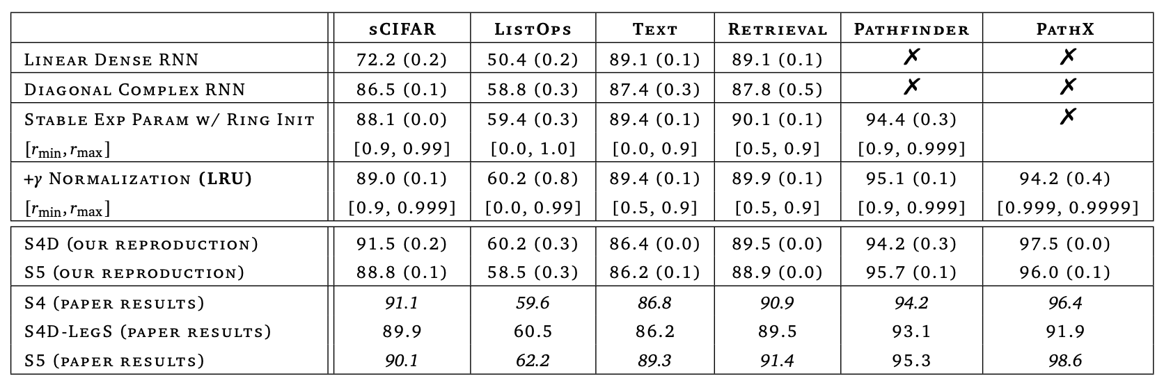
In the original paper, the authors demonstrated how to step-by-step optimize a common RNN through a combination of theory and experiment until achieving near-SOTA results on LRA. This process of analysis and improvement is fascinating and worth savoring. However, since the paper’s experiments were conducted repeatedly on LRA, the experiments themselves are not overly exciting. Here, I only present Table 8 from the paper:

Readers of this article might be more concerned with its performance on NLP, especially the recently popular LM tasks. Unfortunately, the original paper does not cover this. I have conducted some comparative experiments for your reference. The models compared include GAU (same as GAU-\alpha), SA (same as RoFormerV2), LRU, SLRU, and RWKV. Among them, LRU, SLRU, and RWKV only replace the Self-Attention in RoFormerV2 with LRU, SLRU, and RWKV of similar parameter and computation scales. The model parameters are all around 100 million (base version), which is considered small nowadays. All models use DeepNorm for initialization and Tiger as the optimizer. All other hyperparameters are consistent, achieving a relatively strict control of variables.

As can be seen, the ranking in terms of performance is: \text{GAU} > \text{SA} > \text{RWKV} > \text{LRU} > \text{SLRU}

From the experimental results, we can conclude:

1. LRU is superior to SLRU, indicating that introducing complex projection matrices and complex eigenvalues is indeed helpful, though there is a certain loss in computational efficiency (even when keeping the parameter count constant).

2. When the sequence length increases, the performance of the Attention series (GAU, SA) improves, while the performance of the RNN series (LRU, SLRU, RWKV) decreases. This is a fundamental difference between the two, likely because the long-range memory capacity of RNNs is limited by the hidden_size.

3. RWKV may indeed be the best RNN model currently, but there is still a significant gap compared to Attention-class models (GAU, SA).

4. According to point 2, for the RNN series to catch up with the Attention series, the hidden_size may need to be further increased. Thus, in LM tasks, the RNN series might only show an advantage at larger scales.

5. Combining points 1 and 3, could the next improved version of RNN be a complex version of RWKV?

Additionally, there are a few experiences from the experimental process. Since GAU is single-headed, its computational efficiency is significantly better than SA in long-sequence, large-scale scenarios, and its performance is also better. Therefore, GAU should be the best choice for language models within a considerable range—off the top of my head, for parameters under 10 billion and sequence lengths under 5000, GAU is recommended. However, it is undeniable that the RNN series of the same scale is superior in inference efficiency (the calculation amount and cache size per recursive step are consistent), and the training efficiency is not inferior to the Attention series. Therefore, after scaling up the model, there should still be a chance to compete with the Attention series.

It is worth noting that although RWKV performs well overall, there is still a gap compared to GAU and SA. Thus, in a fair comparison, RWKV is not as perfect as rumored. In fact, the RWKV author’s own implementation includes a series of quite obscure tricks said to help enhance LM performance (according to the author, these tricks are the “essence”). These tricks can only be found by reading the author’s source code and were not included in my experiments. It is not ruled out that these tricks help in better training an LM, but I wanted to do a fair controlled experiment rather than actually train a production LM model. Once these tricks are introduced, there are too many variables, and my computing power is limited, making it impossible to compare them one by one.

Of course, the above conclusions are only drawn from “small models” at the 100-million level. I am still trying larger-scale models and cannot give a conclusion for now.

Conclusion

This article introduced an attempt by Google to “save” RNNs, constructing an efficient RNN model from the top down that performs near SOTA on LRA. In addition to the LRA experiments in the original paper, this article also provided my own experimental results on language models, including comparisons with related models like RWKV. Overall, optimized RNN models are not inferior to Attention-class models in training efficiency and offer better inference performance, but there is still a certain gap in language model performance compared to Attention-class models. Perhaps the models need to be made larger to further demonstrate the advantages of RNNs.

Original address: https://kexue.fm/archives/9554

For more details on reprinting, please refer to: Scientific Space FAQ