Recently, I have been experimenting with the Lion optimizer introduced in the post “Google’s New Optimizer Lion: The ’Training Lion’ that Combines Efficiency and Effectiveness.” My interest in Lion stems from the fact that it coincides with some of my previous ideas regarding an ideal optimizer; however, I failed to achieve good results at the time, whereas Lion succeeded.
Compared to the standard Lion, I am more interested in its special case where \beta_1 = \beta_2, which I call “Tiger.” Tiger uses only momentum to construct the update. According to the conclusions in “Gradient Accumulation Hidden in Momentum: Fewer Updates, Better Results?”, in this case, we can implement gradient accumulation “seamlessly” without adding an extra set of parameters! This means that when gradient accumulation is required, Tiger achieves the optimal solution for memory usage. This is also the origin of the name “Tiger” (Tight-fisted Optimizer, an optimizer so stingy it refuses to spend a bit of extra memory).
Furthermore, Tiger incorporates some of our experience in hyperparameter tuning and proposes a simple strategy to prevent the model from producing NaNs (especially during mixed-precision training). Our preliminary experiments show that these modifications in Tiger allow for more user-friendly training of models, especially large ones.
Basic Form
The update rule for Tiger is: \text{Tiger} := \left\{ \begin{aligned} &\boldsymbol{m}_t = \beta \boldsymbol{m}_{t-1} + (1 - \beta) \boldsymbol{g}_t \\ &\boldsymbol{\theta}_t = \boldsymbol{\theta}_{t-1} - \eta_t \left[\text{sign}(\boldsymbol{m}_t) \color{cyan}{ + \lambda_t \boldsymbol{\theta}_{t-1}}\right] \\ \end{aligned} \right. Compared to Lion, it simply chooses parameters \beta_1 = \beta_2 = \beta; compared to SignSGD, it adds momentum and weight decay.
Reference implementation:
The following table compares the update rules of Tiger, Lion, and AdamW:
| Tiger | Lion | AdamW |
|---|---|---|
| \begin{aligned} &\boldsymbol{m}_t = \beta \boldsymbol{m}_{t-1} + (1 - \beta) \boldsymbol{g}_t \\ &\boldsymbol{\theta}_t = \boldsymbol{\theta}_{t-1} - \eta_t [\text{sign}(\boldsymbol{m}_t) \color{cyan}{ + \lambda_t \boldsymbol{\theta}_{t-1}}] \end{aligned} | \begin{aligned} &\boldsymbol{u}_t = \text{sign}(\beta_1 \boldsymbol{m}_{t-1} + (1 - \beta_1) \boldsymbol{g}_t) \\ &\boldsymbol{\theta}_t = \boldsymbol{\theta}_{t-1} - \eta_t (\boldsymbol{u}_t \color{cyan}{ + \lambda_t \boldsymbol{\theta}_{t-1}}) \\ &\boldsymbol{m}_t = \beta_2 \boldsymbol{m}_{t-1} + (1 - \beta_2) \boldsymbol{g}_t \end{aligned} | \begin{aligned} &\boldsymbol{m}_t = \beta_1 \boldsymbol{m}_{t-1} + (1 - \beta_1) \boldsymbol{g}_t\\ &\boldsymbol{v}_t = \beta_2 \boldsymbol{v}_{t-1} + (1 - \beta_2) \boldsymbol{g}_t^2\\ &\hat{\boldsymbol{m}}_t = \boldsymbol{m}_t / (1 - \beta_1^t)\\ &\hat{\boldsymbol{v}}_t = \boldsymbol{v}_t / (1 - \beta_2^t)\\ &\boldsymbol{u}_t = \hat{\boldsymbol{m}}_t / (\sqrt{\hat{\boldsymbol{v}}_t} + \epsilon)\\ &\boldsymbol{\theta}_t = \boldsymbol{\theta}_{t-1} - \eta_t (\boldsymbol{u}_t \color{cyan}{ + \lambda_t \boldsymbol{\theta}_{t-1}}) \end{aligned} |
It is evident that Tiger is the most minimalist among the three.
Hyperparameter Settings
Although Tiger is significantly simplified, there are still several hyperparameters to set: the moving average rate \beta, the learning rate \eta_t, and the weight decay rate \lambda_t. We discuss the selection of these parameters below.
Sliding Rate
The decay rate \beta for the moving average is relatively straightforward. We know that Tiger is equivalent to a special case of Lion where \beta_1 = \beta_2 = \beta. An intuitive choice is \beta = \frac{1}{2}(\beta_1 + \beta_2). In the original Lion paper, for CV tasks, \beta_1=0.9, \beta_2=0.99, so we suggest \beta = 0.945 for CV tasks. For NLP tasks, \beta_1=0.95, \beta_2=0.98, so we suggest \beta = 0.965 for NLP tasks.
Learning Rate
For the learning rate, Tiger draws inspiration from works like Amos and LAMB, setting the learning rate in two different ways. The first category includes bias terms in linear layers and the beta and gamma parameters in Normalization layers. These parameters are characterized by element-wise operations; we suggest setting their learning rate to half of the global relative learning rate \alpha_t. The second category primarily consists of the kernel matrices of linear layers, which perform matrix multiplication with vectors. We suggest setting their learning rate to the global relative learning rate \alpha_t multiplied by the RMS (Root Mean Square) of the parameter itself: \eta_t = \left\{ \begin{aligned} &\alpha_t \times 0.5, & \boldsymbol{\theta} \in \{bias, beta, gamma\} \\[5pt] &\alpha_t \times \text{RMS}(\boldsymbol{\theta}_{t-1}), & \boldsymbol{\theta} \notin \{bias, beta, gamma\} \end{aligned} \right. where \text{RMS}(\boldsymbol{\theta}) = \sqrt{\frac{1}{k}\sum_{i=1}^k \theta_i^2}, \quad \boldsymbol{\theta}=(\theta_1, \theta_2, \dots, \theta_k) The advantage of this setup is that we decouple the scale of the parameters, allowing the learning rate control to be handled by a more universal “global relative learning rate” \alpha_t. This can be roughly understood as the relative learning magnitude per step, a quantity that is not particularly sensitive to the model scale.
In other words, an \alpha_t tuned on a base model can basically be applied to a large model without modification. Note that \alpha_t has a subscript t, so it includes the entire learning rate schedule, including warmup and decay strategies. My experience suggests setting \max(\alpha_t) \in [0.001, 0.002]. As for how to warmup and decay, that depends on your specific task. The Tiger implementation I provided includes a built-in piecewise linear learning rate strategy, which theoretically can simulate any \alpha_t.
Decay Rate
Finally, regarding the weight decay rate \lambda_t, the Lion paper provides some reference settings on its last page. Generally, \lambda_t is set as a constant; I commonly use 0.01. Notably, it is not recommended to apply weight decay to the aforementioned bias, beta, and gamma parameters, or if applied, \lambda_t should be at least an order of magnitude lower. From the perspective of prior distributions, weight decay represents a Gaussian prior on parameters, where \lambda_t is inversely proportional to the parameter variance. Since the variance of bias, beta, and gamma is clearly larger than that of kernel matrices, their \lambda_t should be smaller. \lambda_t = \left\{ \begin{aligned} &0, & \boldsymbol{\theta} \in \{bias, beta, gamma\} \\[5pt] &constant > 0, & \boldsymbol{\theta} \notin \{bias, beta, gamma\} \end{aligned} \right.
Gradient Accumulation
For many readers with limited computing power, increasing the batch size through gradient accumulation is an inevitable step when training large models. Standard gradient accumulation requires an additional set of parameters to cache historical gradients. This means that under gradient accumulation, Adam adds 3 sets of parameters, Lion adds 2 sets, and even AdaFactor without momentum adds 1.x sets (though AdaFactor converges much slower without momentum; adding momentum brings it to 2.x sets).
For Tiger, the update only uses momentum and the original parameters. According to “Gradient Accumulation Hidden in Momentum: Fewer Updates, Better Results?”, we can integrate gradient accumulation into Tiger with the following modification: \text{Tiger} := \left\{ \begin{aligned} &\boldsymbol{m}_t = [(\beta - 1)\chi_{(t-1)/k} + 1] \boldsymbol{m}_{t-1} + \frac{1}{k}(1 - \beta) \boldsymbol{g}_t \\ &\boldsymbol{\theta}_t = \boldsymbol{\theta}_{t-1} - \chi_{t/k}\eta_t [\text{sign}(\boldsymbol{m}_t) \color{cyan}{ + \lambda_t \boldsymbol{\theta}_{t-1}}] \\ \end{aligned} \right. where \chi_{t/k} is the indicator function determining if t is divisible by k: \chi_{t/k} = \left\{ \begin{aligned} &1, \quad t \equiv 0 \pmod k \\ &0, \quad t \not\equiv 0 \pmod k \end{aligned} \right. As we can see, this is equivalent to modifying the sliding average rate \beta and the learning rate \eta_t. It adds almost no memory cost and the entire process is completely “seamless.” This is what I consider the greatest charm of Tiger.
It should be noted that while Lion and Tiger are very similar, Lion cannot achieve this. When \beta_1 \neq \beta_2, Lion’s update requires both the momentum and the current batch’s gradient, which must be cached using different parameters. Tiger’s update only uses momentum, thus satisfying this property. Similarly, the SGDM optimizer can also do this, but it lacks the \text{sign} operation, meaning its learning rate adaptation is insufficient, often leading to unsatisfactory results on models like Transformers (refer to “Why are Adaptive Methods Good for Attention Models?”).
Full and Half Precision
For large models, mixed-precision training is another common “sharp tool” (refer to “Using Mixed Precision and XLA to Accelerate Training in bert4keras”). Mixed precision, simply put, uses half-precision FP16 for model computation and single-precision FP32 for parameter storage and updates. FP32 is used for parameters because of concerns that update magnitudes might be too small, underflowing the FP16 range (roughly 6 \times 10^{-8} \sim 65504), causing some parameters to stop updating and hindering training.
However, Tiger (and Lion) applies the \text{sign} operation to the update, which theoretically allows us to train entirely in half precision! The analysis is straightforward. First, by appropriately scaling the Loss, we can ensure the gradient \boldsymbol{g}_t does not overflow the FP16 range. Since the momentum \boldsymbol{m}_t is just a sliding average of gradients, if the gradient doesn’t overflow, neither will the momentum. \text{sign}(\boldsymbol{m}_t) can only be \pm 1, which certainly won’t overflow. Finally, we only need to ensure the learning rate is not smaller than 6 \times 10^{-8} to prevent the update from underflowing; in practice, we don’t set the learning rate that small. Therefore, Tiger’s entire update process stays within the FP16 range, making full FP16 training theoretically feasible without overflow concerns.
Preventing NaN
However, I found that for the same configuration, training might be normal in FP32 but fail when switching to mixed or half precision. Specifically, the Loss decreases initially, then rises, and finally becomes NaN. We discussed this in “Using Mixed Precision and XLA to Accelerate Training in bert4keras.”. While there are directions for troubleshooting (e.g., adjusting epsilon, infinity values, or loss scaling), sometimes NaNs still occur even after all checks.
Upon debugging, I found that this usually happens when gradients for certain batches become NaN, while the model parameters and forward calculations are still normal. Thus, I devised a simple strategy: if the gradient is NaN, skip the update and slightly contract the parameters: \text{Tiger} := \left\{ \begin{aligned} &\boldsymbol{m}_t = \boldsymbol{m}_{t-1} \\ &\boldsymbol{\theta}_t = (\boldsymbol{\theta}_{t-1} - c) \times s + c \\ \end{aligned} \right. \quad \text{if } \boldsymbol{g}_t = \text{NaN} where s \in (0, 1) represents the contraction rate (I use s=0.99), and c is the initialization center of the parameters (usually 1 for gamma and 0 for others). After this treatment, the loss may rise slightly, but training usually recovers, avoiding a total restart. My experiments show this can alleviate some NaN issues.
Of course, this trick is intended for scenarios where FP32 training is normal and mixed-precision adjustments (epsilon, etc.) have already been made. If the model’s hyperparameters are fundamentally flawed (e.g., the learning rate is too high) such that even FP32 results in NaN, do not expect this trick to solve the problem. Additionally, interested readers could try improving this trick, such as adding a bit of noise after contraction to increase parameter diversity.
Experimental Results
Ignoring the memory optimization from gradient accumulation, Tiger is a special case of Lion. It can be predicted that Tiger’s best performance will not surpass Lion’s best performance. Is the performance drop within an acceptable range? Based on various experimental results so far, my current conclusion is: \begin{aligned} &\text{Performance} \color{red}{(\uparrow)}: \quad \text{Lion} \geq \text{Tiger} \geq \text{AdamW} \approx \text{LAMB} \\ &\text{Memory} \color{red}{(\downarrow)}: \quad \text{Tiger} < \text{Lion} < \text{AdamW} = \text{LAMB} \\ \end{aligned} In other words, Lion is optimal for performance, while Tiger is optimal for memory usage (when gradient accumulation is enabled). In terms of performance, Tiger is not inferior to AdamW, so replacing AdamW with Tiger should not be an issue.
Specific experimental results include several parts. The first part comes from the Lion paper “Symbolic Discovery of Optimization Algorithms.” Figure 12 in the paper compares Lion, Tiger, and AdamW on language models of different sizes:
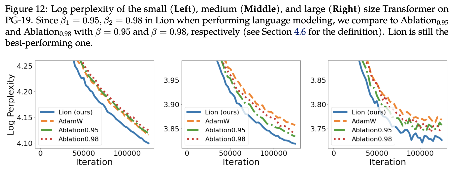
Here, Ablation_{0.95} and Ablation_{0.98} refer to Tiger with \beta set to 0.95 and 0.98, respectively. For small-scale models, both Tiger versions match AdamW, while on middle and large scales, both Tiger versions outperform AdamW. As mentioned earlier, using the mean value \beta=0.965 might yield further improvements.
For CV tasks, the original paper provides Table 7:
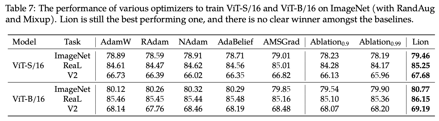
Similarly, Ablation_{0.9} and Ablation_{0.99} refer to Tiger with \beta set to 0.9 and 0.99. In this table, there is a noticeable gap between Tiger and AdamW. However, considering the authors only tested 0.9 and 0.99, and I recommend \beta=0.945, I contacted the authors for supplementary experiments. They replied that with \beta set to 0.92, 0.95, and 0.98, the ImageNet results on ViT-B/16 were all around 80.0%. Comparing this to the figure above, it is certain that with a fine-tuned \beta, Tiger can also match AdamW in CV tasks.
Finally, my own experiments. I frequently use the LAMB optimizer, which performs similarly to AdamW but is more stable and adapts better to different initializations. Notably, LAMB’s learning rate settings can be transferred to Tiger without modification. I retrained the previous base version of the GAU-\alpha model using Tiger. The comparison of training curves is as follows:
As seen, Tiger indeed achieves superior performance compared to LAMB.
Future Work
Is there room for improvement in Tiger? Certainly. There are many ideas, but I haven’t had time to verify them all. Interested readers are welcome to continue this work.
In “Google’s New Optimizer Lion: The ’Training Lion’ that Combines Efficiency and Effectiveness,” I commented on the \text{sign} operation:
Lion treats every component equally through the \text{sign} operation, allowing the model to fully utilize the role of each component, thereby achieving better generalization. In SGD, the update magnitude is proportional to the gradient; however, some components might have small gradients simply because they were poorly initialized, not because they are unimportant. Lion’s \text{sign} operation provides every parameter an opportunity to “regain vitality” or even “create new brilliance.”
However, upon closer reflection, there is room for improvement. “Treating every component equally” is very reasonable at the beginning of training as it preserves as many possibilities for the model as possible. However, if a parameter’s gradient remains very small for a long time, it is likely that the parameter has reached its limit. Continuing to treat it equally might be unfair to the “high-achieving” components with larger gradients and could cause model oscillation.
An intuitive idea is that the optimizer should gradually degrade from Tiger to SGD as training progresses. To this end, we could consider setting the update to: \boldsymbol{u}_t = \text{sign}(\boldsymbol{m}_t) \times |\boldsymbol{m}_t|^{1-\gamma_t} where the absolute value and power operations are element-wise, and \gamma_t is a monotonically decreasing function from 1 to 0. When \gamma_t=1, it corresponds to Tiger; when \gamma_t=0, it corresponds to SGDM.
Readers might complain that this introduces another schedule \gamma_t to tune, making things more complex. This is true if tuned independently. However, recall that (excluding the warmup phase) the relative learning rate \alpha_t is typically a monotonically decreasing function reaching zero. Could we design \gamma_t using \alpha_t? For example, \alpha_t/\alpha_0 is a monotonically decreasing function from 1 to 0. Could it serve as \gamma_t? Perhaps (\alpha_t/\alpha_0)^2 or \sqrt{\alpha_t/\alpha_0} would be better. There is room for tuning, but at least we wouldn’t need to design a completely new schedule spanning the entire training process.
More broadly, since we sometimes use non-monotonic schedules for learning rates (like cosine annealing with restarts), could we use a non-monotonic \gamma_t (equivalent to switching between Tiger and SGDM)? These ideas remain to be verified.
Summary
In this article, we proposed a new optimizer named Tiger (Tight-fisted Optimizer), which simplifies Lion and incorporates our hyperparameter expertise. Notably, in scenarios requiring gradient accumulation, Tiger achieves the theoretical optimal (stingy) solution for memory usage!
Reprinting: Please include the original article address: https://kexue.fm/archives/9512
For more details on reprinting, please refer to: Scientific Space FAQ