Guiding Self-Supervised Learning with the Heat Equation

Basic Equations

As shown in the figure below, the left side represents the solution to the heat equation in physics, while the right side shows attribution heatmaps obtained through saliency methods such as CAM and Integrated Gradients. One can see a certain similarity between the two. Consequently, the authors argue that the heat equation can serve as an important prior for good visual features.

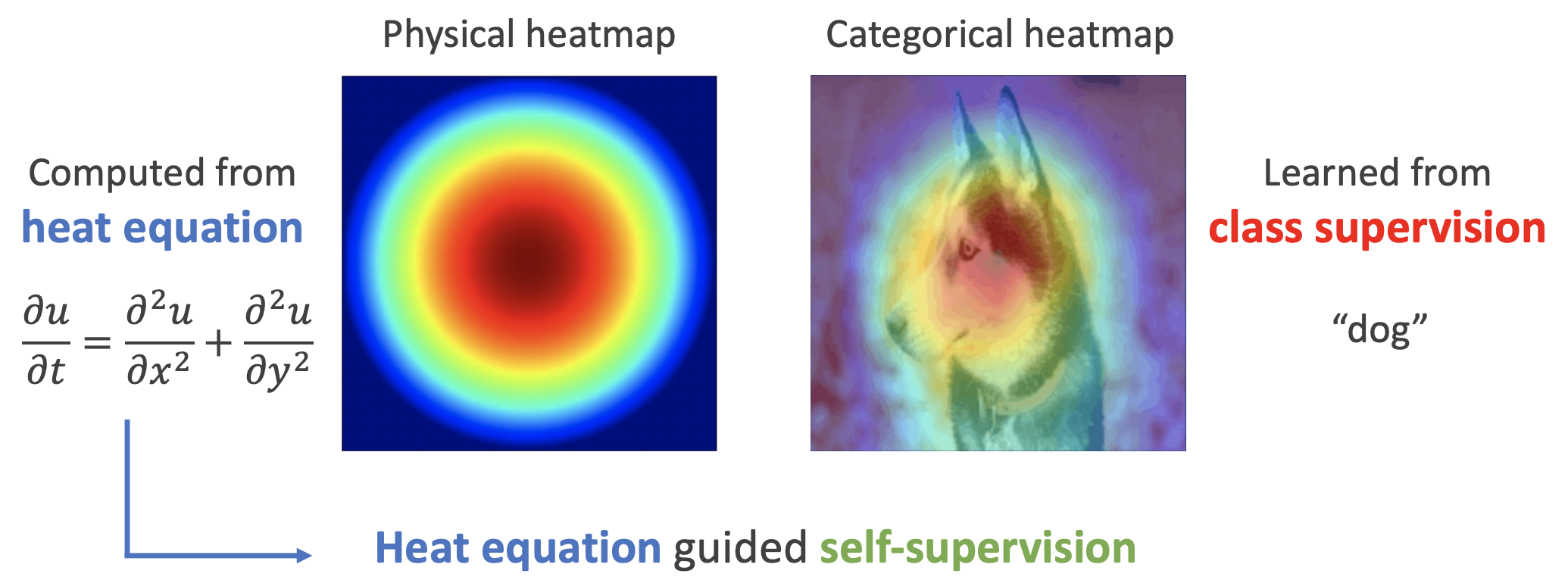
Specifically, the physical heat equation is given by: \begin{equation} \frac{\partial u}{\partial t} = \frac{\partial^2 u}{\partial x^2} + \frac{\partial^2 u}{\partial y^2} \end{equation} where x, y correspond to the "width" and "height" dimensions of the image, and u corresponds to the feature value at that location. Since this work primarily deals with static images rather than video, there is no time dimension t. Thus, we can simply set \frac{\partial u}{\partial t}=0. Since features are typically multi-dimensional vectors rather than scalars, we replace u with \boldsymbol{z}, yielding: \begin{equation} \frac{\partial^2 \boldsymbol{z}}{\partial x^2} + \frac{\partial^2 \boldsymbol{z}}{\partial y^2} = 0 \label{eq:laplace} \end{equation} This is known as the "Laplace equation." It is isotropic, whereas images are not always isotropic. To address this, we can introduce a matrix \boldsymbol{S} to capture this anisotropy: \begin{equation} \frac{\partial^2 \boldsymbol{z}}{\partial x^2} + \boldsymbol{S}\frac{\partial^2 \boldsymbol{z}}{\partial y^2} = 0 \label{eq:laplace-s} \end{equation} However, this is a second-order equation. As we will see later, it is somewhat cumbersome to discretize. Therefore, the authors propose further transforming it into a system of first-order equations: \begin{equation} \frac{\partial \boldsymbol{z}}{\partial x} = \boldsymbol{A}\boldsymbol{z},\quad \frac{\partial \boldsymbol{z}}{\partial y} = \boldsymbol{B}\boldsymbol{z} \label{eq:laplace-1o} \end{equation} It can be verified that if \boldsymbol{S} = -\boldsymbol{A}^2(\boldsymbol{B}^2)^{-1}, then the solution to the above system must also be a solution to equation [eq:laplace-s]. Thus, the original paper takes equation [eq:laplace-1o] as its starting point.

Discrete Reconstruction

Despite the mathematical setup, the core idea of the paper is quite simple: it assumes that the features obtained after passing the original image through an encoder should satisfy equation [eq:laplace-1o] as much as possible. Specifically, after the image passes through the encoder and before global pooling, we obtain a feature map of size w \times h \times d. We view this as m \times n vectors of dimension d, or as a function \boldsymbol{z}(x, y) \in \mathbb{R}^d, where (x, y) is the position of the vector. This function \boldsymbol{z}(x, y) should ideally satisfy equation [eq:laplace-1o].

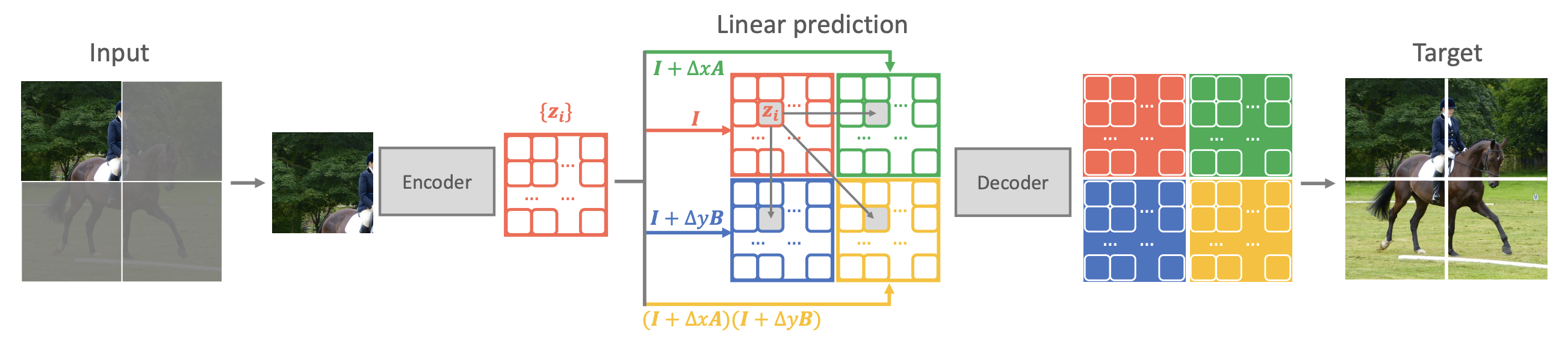
How can we facilitate this? Based on equation [eq:laplace-1o], we can derive a discretization scheme: \begin{equation} \begin{aligned} &\boldsymbol{z}(x+\Delta x, y) \approx \boldsymbol{z}(x, y) + \Delta x \boldsymbol{A}\boldsymbol{z}(x,y) = (\boldsymbol{I} + \Delta x \boldsymbol{A})\boldsymbol{z}(x,y) \\ &\boldsymbol{z}(x, y+\Delta y) \approx \boldsymbol{z}(x, y) + \Delta y \boldsymbol{B}\boldsymbol{z}(x,y) = (\boldsymbol{I} + \Delta y \boldsymbol{B})\boldsymbol{z}(x,y) \end{aligned} \label{eq:laplace-delta} \end{equation} This implies that we can predict the features of neighboring positions using the features at the current position. Consequently, the paper proposes a self-supervised learning method called "QB-Heat":

In each iteration, only a small portion of the image is input. After passing through the encoder to obtain the corresponding features, the features of the full image are predicted via the discretization in [eq:laplace-delta]. These features are then passed into a small decoder to reconstruct the complete image.

The schematic diagram is as follows:

Comparative Analysis

This concludes the introduction to QB-Heat. The remainder of the original paper consists of experimental results and some analyses that (in my opinion) are not highly relevant, so I will skip them here. Interested readers can refer directly to the original paper.

If readers are familiar with the MAE model (refer to "MLM and MAE from the Perspective of Dropout: Some New Inspirations"), they might notice many similarities between QB-Heat and MAE. Both involve inputting a portion of the image into an encoder and then reconstructing the full image, and both utilize a large encoder with a small decoder. Aside from the masking method, the biggest difference lies in the input to the decoder: QB-Heat predicts features for the remaining parts of the image using the approximation in [eq:laplace-delta], whereas MAE simply treats the remaining features as a uniform [MASK] token. It is conceivable that using the approximation in [eq:laplace-delta] is more reasonable than the brute-force filling with [MASK], so it stands to reason that QB-Heat performs better than MAE.

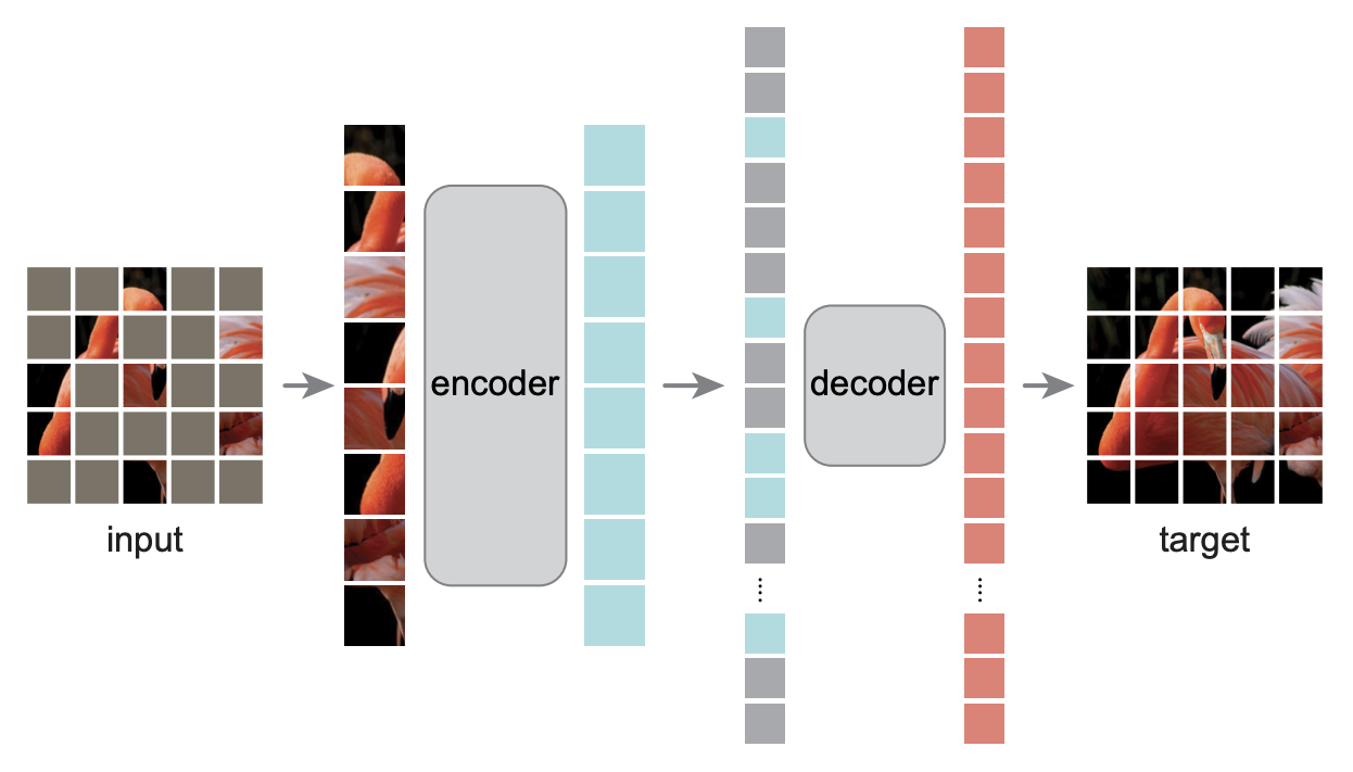
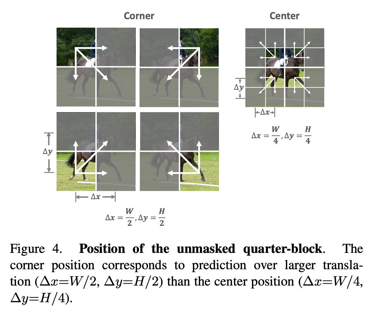
Equation [eq:laplace-delta] dictates that QB-Heat can only predict the surroundings from the center (otherwise, handling interpolation in the middle becomes complicated). Therefore, the masking method for QB-Heat is limited to retaining a continuous square region while masking the periphery, as shown below. Because the input to QB-Heat is a continuous sub-region of the original image, its encoder can be built using either a Transformer or a pure CNN model. In contrast, MAE randomly masks pixels of the original image. To achieve computational savings in the encoder, MAE’s encoder must be a Transformer, as only Transformers can reduce sequence length while preserving positional information.

Personal Thoughts

While the physical perspective is beautiful, it is often just a "pretext" (in a non-pejorative sense). It is more important for us to look through the phenomena to the essence and consider the actual mechanism at work.

First, an obvious point of criticism for QB-Heat is that while the title and method are named after the heat equation, the actual "appearance" of the heat equation lasts less than three seconds, making it feel somewhat optional. In fact, the starting point of the paper should be equation [eq:laplace], the Laplace equation. Although the Laplace equation is formally equivalent to the steady-state solution of the heat equation, they belong to different branches in both mathematical and physical classification and research. Thus, the name "heat equation" feels a bit forced. Secondly, the Laplace equation is not used in its original form [eq:laplace] or [eq:laplace-s], but rather in the simplified form [eq:laplace-1o], and applied via the approximation [eq:laplace-delta]. Setting aside the physical background and looking directly at equation [eq:laplace-delta], it states the following hypothesis:

Adjacent feature vectors should be as similar as possible, and the difference between them should ideally be accounted for by the same linear transformation.

In short, it makes explicit predictions for feature vectors through assumptions of continuity and linearity, thereby acting as an implicit regularizer. This reminds me of mixup, which also adds implicit linear regularization to the model by explicitly constructing data, thereby enhancing the model’s final generalization ability.

For me, when I see a method in Computer Vision (CV), I usually wonder if it can be transferred to NLP. Is such a transfer possible for QB-Heat? Compared to MAE, the most significant change QB-Heat makes is that the features of the remaining parts of the original image should be predicted based on certain assumptions, rather than being replaced uniformly by [MASK]. QB-Heat uses continuity and linearity assumptions for CV; can this be replicated for NLP? Language is essentially a time series with only one variation dimension, which is equivalent to asking whether we can assume that the sentence vectors between adjacent sentences differ by the same linear transformation? It seems that natural language should not possess such good continuity, but from the perspective of linear regularization, it might not be unfeasible, as mixup has worked well in many NLP tasks.

Additionally, if we randomly mask a portion of tokens instead of retaining a continuous sub-interval like QB-Heat, it seems we could directly use the feature vectors from both sides to perform linear interpolation to predict the features of the middle positions. This would also satisfy the continuity and linearity assumptions. I wonder if this approach would yield better results? These are preliminary thoughts that await experimental verification.

Article Summary

This article introduced QB-Heat, a scheme that uses the heat equation to guide self-supervised learning. The difference between it and MAE is the use of simple predictions rather than [MASK] tokens as the features for the remaining parts of the image passed to the decoder.

Reprinted from: https://kexue.fm/archives/9359

For more detailed reprinting matters, please refer to: "Scientific Space FAQ"