Text similarity is generally approached in two ways: "interactive" (cross-encoders) and "feature-based" (bi-encoders). Many readers are likely familiar with these concepts; I previously wrote an article "CoSENT (II): How Big is the Gap Between Feature-based and Interactive Matching?" to compare their performance. In general, interactive similarity models usually yield better results, but using them directly for large-scale retrieval is impractical. Conversely, feature-based similarity offers faster retrieval speeds but slightly inferior performance.
Therefore, how to improve the retrieval speed of interactive similarity models while maintaining their performance is a subject of ongoing research in academia. Recently, the paper "Efficient Nearest Neighbor Search for Cross-Encoder Models using Matrix Factorization" proposed a new answer: CUR decomposition.
Problem Analysis
In a retrieval scenario, we typically have a massive candidate set \mathcal{K}. Without loss of generality, we can assume \mathcal{K} is constant. The task of retrieval is to find the several results k \in \mathcal{K} most relevant to an arbitrary request q \in \mathcal{Q}. Interactive similarity models directly train a relevance scoring function s(q, k). Theoretically, we could calculate s(q, k) for every k \in \mathcal{K} and then sort them in descending order. However, this means the computational complexity for each retrieval is \mathcal{O}(|\mathcal{K}|), and intermediate results cannot be cached, making the cost unacceptable.
Acceptable computational complexity is found in similarity measures with a matrix factorization form. For a single sample, this refers to inner-product-based similarity and its variants. A classic implementation involves an encoder \boldsymbol{E} that encodes q and k into two vectors \boldsymbol{E}(q) and \boldsymbol{E}(k), followed by calculating the inner product \boldsymbol{E}(q)^{\top}\boldsymbol{E}(k); this is feature-based similarity. Such a scheme has several characteristics: 1. All \boldsymbol{E}(k) can be pre-calculated and cached; 2. The inner product of \boldsymbol{E}(q) with all \boldsymbol{E}(k) can be converted into matrix multiplication, allowing for fully parallelized and fast computation; 3. Retrieval speed can be further enhanced using tools like Faiss with approximate algorithms.
Thus, the idea for accelerating interactive similarity retrieval is to transform it into a matrix factorization form. A classic implementation involves using a feature-based similarity model to distill and learn the effects of an interactive model. The ingenuity of this Google paper lies in not introducing any new models, but directly utilizing CUR decomposition on the original interactive similarity model to achieve acceleration. This scheme is named ANNCUR.
Matrix Factorization
CUR decomposition is a type of matrix factorization. When matrix factorization is mentioned, many readers’ first reaction might be SVD. In fact, the reason everyone is so sensitive to SVD is not that it is particularly intuitive, but because it is frequently introduced. In terms of being intuitive and easy to understand, CUR decomposition is clearly superior.
Actually, we can understand SVD and CUR decomposition from a unified perspective: for a scoring function s(q, k), we hope to construct the following approximation: s(q,k) \approx \sum_{u\in\mathcal{U},v\in\mathcal{V}} f(q, u) g(u, v) h(v, k)\label{eq:decom} Generally, there are constraints |\mathcal{U}|, |\mathcal{V}| \ll |\mathcal{Q}|, |\mathcal{K}|, making it a compressed decomposition. We can view \mathcal{U} as a "representative set" (or "cluster centers") of \mathcal{K}, and similarly \mathcal{V} as a "representative set" of \mathcal{Q}. Then the above decomposition becomes very vivid:
The score s(q, k) of q and k is approximated by first calculating the score f(q, u) between q and the "representatives" u \in \mathcal{U} of \mathcal{K}, then calculating the score h(v, k) between k and the "representatives" v \in \mathcal{V} of \mathcal{Q}, and finally performing a weighted sum using weights g(u, v).
In other words, the direct interaction between q and k is transformed into their respective interactions with "representatives," followed by weighting the results. The advantage of this is obvious: once f, g, h are determined, all g(u, v) and h(v, k) can be pre-calculated and cached as a matrix. For each retrieval, we only need to calculate f(q, u) for |\mathcal{U}| times and then perform one matrix multiplication (inner-product-based retrieval). Thus, the computational complexity of retrieval is transformed from \mathcal{O}(|\mathcal{K}|) to \mathcal{O}(|\mathcal{U}|) (with tools like Faiss, inner-product-based retrieval can be optimized to approximately \mathcal{O}(1), and thus can be ignored).
Assuming the request set \mathcal{Q} is also finite, then all s(q, k) constitute a |\mathcal{Q}| \times |\mathcal{K}| matrix \boldsymbol{S}. Correspondingly, f(q, u), g(u, v), h(v, k) correspond to a |\mathcal{Q}| \times |\mathcal{U}| matrix \boldsymbol{F}, a |\mathcal{U}| \times |\mathcal{V}| matrix \boldsymbol{G}, and a |\mathcal{V}| \times |\mathcal{K}| matrix \boldsymbol{H}. Equation [eq:decom] becomes a matrix decomposition: \begin{array}{ccccc} \boldsymbol{S} & \approx & \boldsymbol{F} & \boldsymbol{G} & \boldsymbol{H} \\ \in\mathbb{R}^{|\mathcal{Q}|\times |\mathcal{K}|} & & \in\mathbb{R}^{|\mathcal{Q}|\times |\mathcal{U}|} & \in\mathbb{R}^{|\mathcal{U}|\times |\mathcal{V}|} & \in\mathbb{R}^{|\mathcal{V}|\times |\mathcal{K}|} \end{array}\label{eq:m-decom}
CUR Decomposition
If \boldsymbol{G} is restricted to be a diagonal matrix while \boldsymbol{F} and \boldsymbol{H} have no special restrictions, the corresponding decomposition is SVD. SVD is equivalent to creating several virtual "representatives," which results in a better fit, but it is difficult for us to understand the specific meaning of these "representatives" constructed by the algorithm—meaning its interpretability is somewhat poor.
CUR decomposition is more intuitive. it posits that "representatives" should be members of the original population. That is, the representatives of \mathcal{Q} and \mathcal{K} should be subsets selected from the sets themselves, i.e., \mathcal{U} \subset \mathcal{K}, \mathcal{V} \subset \mathcal{Q}. Consequently, (q, u) and (v, k) are among the original (q, k) pairs, so the original scoring function s can be used: s(q,k) \approx \sum_{u\in\mathcal{U},v\in\mathcal{V}} s(q, u) g(u, v) s(v, k) Thus, the only function to be determined is g(u, v). From the perspective of matrix decomposition, \boldsymbol{F} in Equation [eq:m-decom] is a submatrix composed of several columns of \boldsymbol{S}, and \boldsymbol{H} is a submatrix composed of several rows of \boldsymbol{S}. The remaining task is to calculate matrix \boldsymbol{G}. The calculation of \boldsymbol{G} is also intuitive. Let’s first consider a very special case where \mathcal{U} = \mathcal{K}, \mathcal{V} = \mathcal{Q} and |\mathcal{Q}| = |\mathcal{K}|. In this case, the CUR decomposition is \boldsymbol{S} \approx \boldsymbol{S}\boldsymbol{G}\boldsymbol{S}, where \boldsymbol{S} and \boldsymbol{G} are square matrices. Since we have taken the entirety of \mathcal{Q} and \mathcal{K} as representatives, we naturally hope for = instead of \approx. If we take =, we can directly solve for \boldsymbol{G} = \boldsymbol{S}^{-1}.
However, this implies that \boldsymbol{S} must be invertible, which is not always true. In such cases, the matrix inverse operation must be generalized, which we call the "pseudo-inverse," denoted as \boldsymbol{G} = \boldsymbol{S}^{\dagger}. Specifically, the pseudo-inverse is also defined for non-square matrices; therefore, when |\mathcal{Q}| \neq |\mathcal{K}|, we can similarly solve for \boldsymbol{G} = \boldsymbol{S}^{\dagger}. Finally, when \mathcal{U} \neq \mathcal{K} or \mathcal{V} \neq \mathcal{Q}, the result is similar, except the matrix for which the pseudo-inverse is calculated is replaced by the intersection matrix of \boldsymbol{F} and \boldsymbol{H} (i.e., the \mathcal{U} \times \mathcal{V} matrix formed by the intersection of several rows and columns of \boldsymbol{S}): \boldsymbol{S} \approx \boldsymbol{F} (\boldsymbol{F}\cap \boldsymbol{H})^{\dagger}\boldsymbol{H}
The entire process is illustrated in the figure below:
Accelerating Retrieval
This is not the first time CUR decomposition has been discussed here. An article from early last year, "Nyströmformer: A Linearized Attention Scheme Based on Matrix Decomposition", introduced Nyströmformer, which is also designed based on the idea of CUR decomposition. The original paper spent considerable space introducing CUR decomposition. ANNCUR uses CUR decomposition for retrieval acceleration, showing that CUR has broad applications.
The principle of acceleration was briefly mentioned earlier; let’s summarize it now. First, we select several representative q \in \mathcal{V} \subset \mathcal{Q} and k \in \mathcal{U} \subset \mathcal{K}, calculate their pairwise scores to form the matrix \boldsymbol{F} \cap \boldsymbol{H}, and obtain matrix \boldsymbol{G} after calculating the pseudo-inverse. Then, we pre-calculate the scoring matrix between q \in \mathcal{V} and k \in \mathcal{K} and store \boldsymbol{G}\boldsymbol{H}. Finally, for each query q, we calculate scores with every k \in \mathcal{U} to get a |\mathcal{U}|-dimensional vector, and then multiply this vector by the cached matrix \boldsymbol{G}\boldsymbol{H} to obtain the scoring vector for q and every k \in \mathcal{K}.
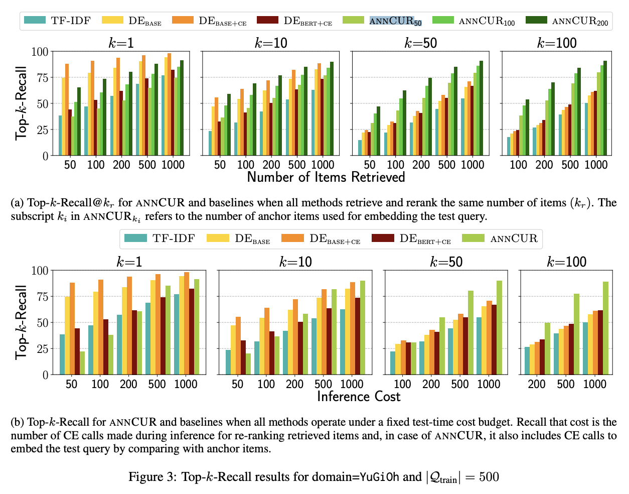
This is the general principle of ANNCUR. For specific details, readers can refer to the original paper, such as why replacing the interactive similarity model with the [EMB]-CE version mentioned in the paper yields better results. Some readers might ask, "How should the representative q, k be selected?" In fact, in most cases, they are selected randomly. This leaves some room for improvement; for example, one could select the ones closest to cluster centers after clustering. These are left for everyone to explore. Additionally, it should be noted that CUR decomposition itself is an approximation and inevitably has errors. Therefore, this acceleration scheme is primarily designed for retrieval scenarios. The characteristic of retrieval is a focus on top-k recall rather than strictly requiring top-1 precision. We can use CUR decomposition acceleration to recall several results and then use the precise s(q, k) for a re-ranking to improve accuracy.
Summary
This article reviewed CUR decomposition in matrix factorization and introduced its application in accelerating interactive similarity retrieval.
When reposting, please include the original address: https://kexue.fm/archives/9336
For more detailed reposting matters, please refer to: "Scientific Space FAQ"