Old readers might notice that, compared to the previous update frequency, this article is "long overdue." This is because I have been "thinking too much" about this topic.
Through the previous nine articles, we have provided a relatively comprehensive introduction to generative diffusion models. Although there is a lot of theoretical content, we can observe that the diffusion models introduced previously all deal with continuous objects and are built upon the forward process of adding Gaussian noise. This article, born from "thinking too much," aims to construct a Unified Diffusion Model (UDM) framework that can break through the aforementioned limitations:
1. No restriction on object types (can be continuous \boldsymbol{x} or discrete \boldsymbol{x});
2. No restriction on the forward process (the forward process can be constructed using various transformations such as adding noise, blurring, masking, or deletion);
3. No restriction on time types (can be discrete time t or continuous time t);
4. Inclusion of existing results (can derive previous results such as DDPM, DDIM, SDE, ODE, etc.).
Is this too "fanciful"? Is there such an ideal framework? This article attempts to explore this.
Forward Process
From the previous series of introductions, we know that constructing a diffusion model involves three parts: the "forward process," the "reverse process," and the "training objective." In this section, we analyze the "forward process."
In the original DDPM, we described the forward process through p(\boldsymbol{x}_t|\boldsymbol{x}_{t-1}). Later, with the publication of works like DDIM, we gradually realized that the training objective and the generation process of diffusion models are not directly related to p(\boldsymbol{x}_t|\boldsymbol{x}_{t-1}). Instead, the connection with p(\boldsymbol{x}_t|\boldsymbol{x}_0) is more direct, and deriving p(\boldsymbol{x}_t|\boldsymbol{x}_0) from p(\boldsymbol{x}_t|\boldsymbol{x}_{t-1}) is often difficult. Therefore, a more practical operation is to start directly from p(\boldsymbol{x}_t|\boldsymbol{x}_0), treating p(\boldsymbol{x}_t|\boldsymbol{x}_0) as the forward process.
The most direct role of p(\boldsymbol{x}_t|\boldsymbol{x}_0) is to construct the training data for the diffusion model. Thus, the most basic requirement for p(\boldsymbol{x}_t|\boldsymbol{x}_0) is that it must be easy to sample from. To this end, we can use reparameterization: \boldsymbol{x}_t = \boldsymbol{\mathcal{F}}_t(\boldsymbol{x}_0,\boldsymbol{\varepsilon})\label{eq:re-param} where \boldsymbol{\mathcal{F}} is a deterministic function of t, \boldsymbol{x}_0, \boldsymbol{\varepsilon}, and \boldsymbol{\varepsilon} is a random variable sampled from some standard distribution q(\boldsymbol{\varepsilon}). A common choice is the standard normal distribution, but other distributions are usually feasible. One can imagine that this form contains sufficiently rich transformations from \boldsymbol{x}_0 to \boldsymbol{x}_t, and it imposes no constraints on the data types of \boldsymbol{x}_0 and \boldsymbol{x}_t. Generally, the only restriction is that the smaller t is, the more complete the information of \boldsymbol{x}_0 contained in \boldsymbol{\mathcal{F}}_t(\boldsymbol{x}_0,\boldsymbol{\varepsilon}) is. In other words, reconstructing \boldsymbol{x}_0 using \boldsymbol{\mathcal{F}}_t(\boldsymbol{x}_0,\boldsymbol{\varepsilon}) is easier for smaller t. Conversely, reconstruction becomes more difficult as t increases, until at some upper bound T, the information of \boldsymbol{x}_0 in \boldsymbol{\mathcal{F}}_T(\boldsymbol{x}_0,\boldsymbol{\varepsilon}) almost disappears, and reconstruction becomes nearly impossible.
Reverse Process
The reverse process of a diffusion model gradually generates realistic data through multi-step iterations, the key to which is the probability distribution p(\boldsymbol{x}_{t-1}|\boldsymbol{x}_t). Generally, we have: p(\boldsymbol{x}_{t-1}|\boldsymbol{x}_t) = \int p(\boldsymbol{x}_{t-1}|\boldsymbol{x}_t, \boldsymbol{x}_0) p(\boldsymbol{x}_0|\boldsymbol{x}_t) d\boldsymbol{x}_0\label{eq:p-factor} If \boldsymbol{x}_0 is discrete data, the integral is replaced by a summation. The basic requirement for p(\boldsymbol{x}_{t-1}|\boldsymbol{x}_t) is also ease of sampling. Therefore, we require p(\boldsymbol{x}_{t-1}|\boldsymbol{x}_t, \boldsymbol{x}_0) and p(\boldsymbol{x}_0|\boldsymbol{x}_t) to be easy to sample from. In this way, we can complete the sampling of p(\boldsymbol{x}_{t-1}|\boldsymbol{x}_t) through the following process: \hat{\boldsymbol{x}}_0\sim p(\boldsymbol{x}_0|\boldsymbol{x}_t)\quad \& \quad \boldsymbol{x}_{t-1}\sim p(\boldsymbol{x}_{t-1}|\boldsymbol{x}_t, \boldsymbol{x}_0=\hat{\boldsymbol{x}}_0) \quad \Rightarrow \quad \boldsymbol{x}_{t-1}\sim p(\boldsymbol{x}_{t-1}|\boldsymbol{x}_t) From this decomposition, each step of the \boldsymbol{x}_t\to \boldsymbol{x}_{t-1} sampling actually consists of two sub-steps:
1. Prediction: Make a simple "prediction" of \boldsymbol{x}_0 using p(\boldsymbol{x}_0|\boldsymbol{x}_t);
2. Correction: Integrate the prediction result using p(\boldsymbol{x}_{t-1}|\boldsymbol{x}_t, \boldsymbol{x}_0) to push the estimate one small step forward.
Thus, the reverse process of a diffusion model is a repeated "predict-correct" process. By continuously integrating the prediction results of \boldsymbol{x}_t\to \boldsymbol{x}_0, we obtain a progressively corrected sequence \boldsymbol{x}_T\to\cdots\to\boldsymbol{x}_t\to \boldsymbol{x}_{t-1}\to\cdots\to \boldsymbol{x}_0, decomposing a generation task that was originally difficult to achieve in one step into multiple steps.
Training Objective
Of course, the current reverse process is still just "theory on paper" because we know nothing about p(\boldsymbol{x}_{t-1}|\boldsymbol{x}_t, \boldsymbol{x}_0) and p(\boldsymbol{x}_0|\boldsymbol{x}_t). In this section, we first discuss p(\boldsymbol{x}_0|\boldsymbol{x}_t).
Clearly, p(\boldsymbol{x}_0|\boldsymbol{x}_t) is a probabilistic model that uses \boldsymbol{x}_t to predict \boldsymbol{x}_0. We need to estimate it using a distribution that is "easy to sample and easy to calculate." When \boldsymbol{x}_0 is continuous data, our choices are limited, usually a normal distribution with a trainable mean: p(\boldsymbol{x}_0|\boldsymbol{x}_t) \approx q(\boldsymbol{x}_0|\boldsymbol{x}_t) = \mathcal{N}(\boldsymbol{x}_0;\boldsymbol{\mathcal{G}}_t(\boldsymbol{x}_t),\bar{\sigma}_t^2 \boldsymbol{I})\label{eq:normal} To reduce training difficulty, we generally do not treat the variance \bar{\sigma}_t^2 as a trainable parameter, but instead estimate it post-hoc using the method in "Generative Diffusion Models Part 7: Optimal Diffusion Variance Estimation (Part 1)". On the other hand, when \boldsymbol{x}_0 is discrete data, we can model it using autoregressive or non-autoregressive language models (Seq2Seq). Discrete probability modeling and sampling are relatively easier.
With the specific form of the approximate distribution q(\boldsymbol{x}_0|\boldsymbol{x}_t), the training objective is simple. A natural choice is cross-entropy: \mathbb{E}_{\boldsymbol{x}_0\sim \tilde{p}(\boldsymbol{x}_0),\boldsymbol{x}_t\sim p(\boldsymbol{x}_t|\boldsymbol{x}_0)}[-\log q(\boldsymbol{x}_0|\boldsymbol{x}_t)] = \mathbb{E}_{\boldsymbol{x}_0\sim \tilde{p}(\boldsymbol{x}_0),\boldsymbol{\varepsilon}\sim q(\boldsymbol{\varepsilon})}[-\log q(\boldsymbol{x}_0|\boldsymbol{\mathcal{F}}_t(\boldsymbol{x}_0,\boldsymbol{\varepsilon}))] This solves the problem of estimating p(\boldsymbol{x}_0|\boldsymbol{x}_t) and designing the training objective. If q(\boldsymbol{x}_0|\boldsymbol{x}_t) is the standard normal distribution in Eq. \eqref{eq:normal}, then the result after omitting constants is: \mathbb{E}_{\boldsymbol{x}_0\sim \tilde{p}(\boldsymbol{x}_0),\boldsymbol{\varepsilon}\sim q(\boldsymbol{\varepsilon})}\left[\frac{1}{2\bar{\sigma}_t^2}\Vert\boldsymbol{x}_0 - \boldsymbol{\mathcal{G}}_t(\boldsymbol{\mathcal{F}}_t(\boldsymbol{x}_0,\boldsymbol{\varepsilon}))\Vert^2\right]
Conditional Probability
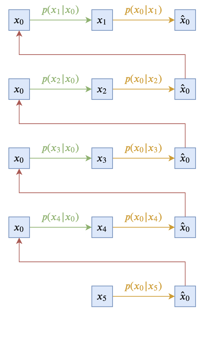
Now only p(\boldsymbol{x}_{t-1}|\boldsymbol{x}_t, \boldsymbol{x}_0) remains, which is the probability of predicting \boldsymbol{x}_{t-1} given \boldsymbol{x}_t, \boldsymbol{x}_0. This probability distribution also has some design space, provided it satisfies the marginal distribution identity: \int p(\boldsymbol{x}_{t-1}|\boldsymbol{x}_t, \boldsymbol{x}_0)p(\boldsymbol{x}_t|\boldsymbol{x}_0) d\boldsymbol{x}_t= p(\boldsymbol{x}_{t-1}|\boldsymbol{x}_0)\label{eq:margin} Obviously, a simplest choice that satisfies this equation is to directly take: p(\boldsymbol{x}_{t-1}|\boldsymbol{x}_t, \boldsymbol{x}_0) = p(\boldsymbol{x}_{t-1}|\boldsymbol{x}_0) That is, making p(\boldsymbol{x}_{t-1}|\boldsymbol{x}_t, \boldsymbol{x}_0) independent of \boldsymbol{x}_t. Such a diffusion model can be described by the following two diagrams (using T=5 as an example):
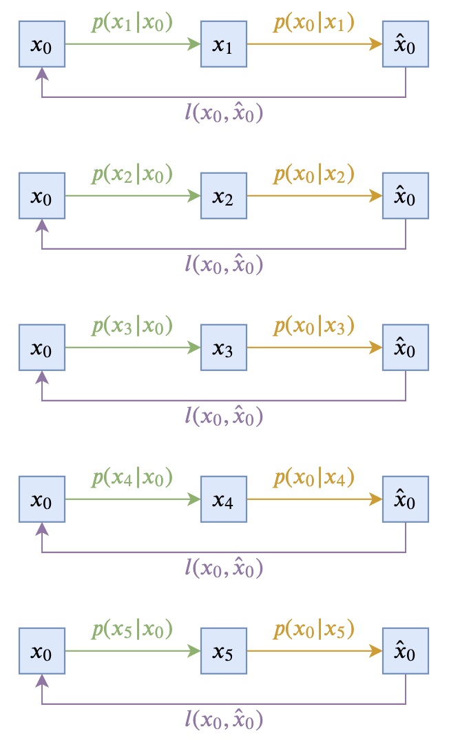
This minimalist choice is theoretically sound; however, the practical effect is usually not very good because \boldsymbol{x}_{t-1} depends entirely on \boldsymbol{x}_0. Since \boldsymbol{x}_0 represents the original real sample, in the reverse process, we can only sample via the approximate distribution q(\boldsymbol{x}_0|\boldsymbol{x}_t), which is usually not accurate enough, leading to continuous error accumulation. Additionally, p(\boldsymbol{x}_{t-1}|\boldsymbol{x}_0) introduces noise during the sampling process, which might severely damage the information of the just-predicted \hat{\boldsymbol{x}}_0, thereby degrading the generation quality.
Fortunately, in most cases, we can derive a new result based on the simple choice p(\boldsymbol{x}_{t-1}|\boldsymbol{x}_t, \boldsymbol{x}_0) = p(\boldsymbol{x}_{t-1}|\boldsymbol{x}_0). According to Eq. \eqref{eq:re-param}, we know: \begin{aligned} \boldsymbol{x}_{t-1} \sim p(\boldsymbol{x}_{t-1}|\boldsymbol{x}_0)\quad\Leftrightarrow&\,\quad\boldsymbol{x}_{t-1} = \boldsymbol{\mathcal{F}}_{t-1}(\boldsymbol{x}_0,\boldsymbol{\varepsilon}) \\ \boldsymbol{x}_t \sim p(\boldsymbol{x}_t|\boldsymbol{x}_0)\quad\Leftrightarrow&\,\quad\boldsymbol{x}_t = \boldsymbol{\mathcal{F}}_t(\boldsymbol{x}_0,\boldsymbol{\varepsilon}) \end{aligned} Assuming \boldsymbol{\mathcal{F}}_t(\boldsymbol{x}_0,\boldsymbol{\varepsilon}) is invertible with respect to \boldsymbol{\varepsilon}, we can solve for \boldsymbol{\varepsilon} = \boldsymbol{\mathcal{F}}_t^{-1}(\boldsymbol{x}_0,\boldsymbol{x}_t). At this point, we can replace \boldsymbol{\varepsilon} in \boldsymbol{\mathcal{F}}_{t-1}(\boldsymbol{x}_0,\boldsymbol{\varepsilon}) with this solved \boldsymbol{\varepsilon}, yielding: \boldsymbol{x}_{t-1} = \boldsymbol{\mathcal{F}}_{t-1}(\boldsymbol{x}_0,\boldsymbol{\mathcal{F}}_t^{-1}(\boldsymbol{x}_0,\boldsymbol{x}_t)) This is equivalent to: p(\boldsymbol{x}_{t-1}|\boldsymbol{x}_t, \boldsymbol{x}_0) = \delta\big(\boldsymbol{x}_{t-1} - \boldsymbol{\mathcal{F}}_{t-1}(\boldsymbol{x}_0,\boldsymbol{\mathcal{F}}_t^{-1}(\boldsymbol{x}_0,\boldsymbol{x}_t))\big) This is a design for p(\boldsymbol{x}_{t-1}|\boldsymbol{x}_t, \boldsymbol{x}_0) that depends on both \boldsymbol{x}_t and \boldsymbol{x}_0. Here, \boldsymbol{x}_t shares part of the dependence of \boldsymbol{x}_{t-1} on \boldsymbol{x}_0 and eliminates noise, allowing the "progress" of each generation step to accumulate stably. Therefore, the reverse process using this design often yields better results.
Furthermore, if q(\boldsymbol{\varepsilon}) is a standard normal distribution, we can obtain even more general results. Due to the additivity of normal distributions, we have: \boldsymbol{x}_{t-1} = \boldsymbol{\mathcal{F}}_{t-1}(\boldsymbol{x}_0,\boldsymbol{\varepsilon})\quad\Leftrightarrow\quad\boldsymbol{x}_{t-1} = \boldsymbol{\mathcal{F}}_{t-1}(\boldsymbol{x}_0,\sqrt{1 - \tilde{\sigma}_t^2}\boldsymbol{\varepsilon}_1 + \tilde{\sigma}_t \boldsymbol{\varepsilon}_2) In this way, the \boldsymbol{\varepsilon} solved from \boldsymbol{x}_0, \boldsymbol{x}_t can be used to replace only one of \boldsymbol{\varepsilon}_1 or \boldsymbol{\varepsilon}_2. The resulting sampling process for p(\boldsymbol{x}_{t-1}|\boldsymbol{x}_t, \boldsymbol{x}_0) is: \quad\boldsymbol{x}_{t-1} = \boldsymbol{\mathcal{F}}_{t-1}(\boldsymbol{x}_0,\sqrt{1 - \tilde{\sigma}_t^2}\boldsymbol{\mathcal{F}}_t^{-1}(\boldsymbol{x}_0,\boldsymbol{x}_t) + \tilde{\sigma}_t \boldsymbol{\varepsilon})
Reflection and Analysis
At this point, the theoretical framework of the Unified Diffusion Model (UDM) has been constructed. In the next article, we will introduce how to derive existing diffusion model results from the UDM framework through specific examples, as well as obtain some new results. In this section, we reflect on the reasoning of the entire text.
After reading the full text, many readers might be confused because the results here are based on a unified framework summarized from my previous understanding of all diffusion models. The overall technique is not very difficult, but the logic is not easy to straighten out. First, the goal of this article is to "design a unified theoretical framework for diffusion models" that can achieve the goals listed at the beginning. The key to "design" is grasping "freedom" and "constraints"—some parts can be chosen flexibly, while others are constrained and cannot be handled arbitrarily.
If readers are already familiar with existing generative diffusion models, they should realize that the essential idea of diffusion models is "learning to construct from destruction." Therefore, the method of "destruction" can theoretically be chosen arbitrarily, while "construction" is what needs to be learned. Of course, the method of "destruction" is not entirely unconstrained; generally, it must be "progressive destruction" so that we can learn "progressive construction." Thus, we constructed the destruction process (forward process) in Eq. \eqref{eq:re-param}, where t describes the progress of destruction, \mathcal{F} represents any destruction method, and there are no special restrictions on the original data \boldsymbol{x}_0. As for \boldsymbol{\varepsilon}, it describes the random factors that may exist in the destruction process. In this way, we have established a most general destruction process.
As for construction, we first provided the decomposition in Eq. \eqref{eq:p-factor}, which is an identity given by probability theory itself. We can understand it as a constraint or as a guide. How did I know to think of Eq. \eqref{eq:p-factor}? In hindsight, the forward process is an \boldsymbol{x}_0\to \boldsymbol{x}_t process, so the reverse process should be linked to \boldsymbol{x}_t\to \boldsymbol{x}_0 as much as possible, leading to the connection with Eq. \eqref{eq:p-factor}.
The decomposition in Eq. \eqref{eq:p-factor} contains two parts. p(\boldsymbol{x}_0|\boldsymbol{x}_t) is already clear: it is the probability of using \boldsymbol{x}_t to predict \boldsymbol{x}_0. This part obviously has no room for further simplification and must be modeled directly. The other part, p(\boldsymbol{x}_{t-1}|\boldsymbol{x}_t, \boldsymbol{x}_0), falls into the category of "free design." It requires ease of sampling, and its "constraint" is given by the identity in Eq. \eqref{eq:margin}, which is also from probability theory. As for the subsequent process of designing p(\boldsymbol{x}_{t-1}|\boldsymbol{x}_t, \boldsymbol{x}_0) under this constraint, it indeed involves some skill. There are no shortcuts here; I also spent a long time thinking about it in conjunction with existing diffusion model works before clarifying the process.
In general, when designing a model, one must always know what they want ("freedom") and what the limitations of those desires are ("constraints"). Under the premise of clarifying "freedom" and "constraints," one should try to draw on existing work and theoretical foundations to move closer to the goal.
Conclusion
This article constructs a new theoretical framework for diffusion models (Unified Diffusion Model, UDM). Theoretically, it can encompass existing generative diffusion model results and allows for more general diffusion methods and data types. Specific examples will be introduced in the next article.
Reprinted from: https://kexue.fm/archives/9262