Many readers may have heard of or even read Felix Klein’s book series "Elementary Mathematics from a Higher Standpoint". As the name suggests, this involves re-examining previously learned elementary mathematics from a deeper, more complete mathematical perspective to gain a more comprehensive understanding and even achieve the effect of "learning new things by reviewing the old." Similar books include "Overcoming Calculus" and "Visual Complex Analysis".
Returning to diffusion models, we have already interpreted DDPM from different perspectives through three articles. Does it also have a "higher perspective" for understanding that can provide new insights? Certainly. The DDIM model introduced in "Denoising Diffusion Implicit Models" is a classic case. In this article, we will explore it together.
Analysis of Ideas
In "Generative Diffusion Models (Part 3): DDPM = Bayes + Denoising", we mentioned that the derivation introduced there is closely related to DDIM. Specifically, the derivation route of that article can be summarized as follows: p(\boldsymbol{x}_t|\boldsymbol{x}_{t-1}) \xrightarrow{\text{Derive}} p(\boldsymbol{x}_t|\boldsymbol{x}_0) \xrightarrow{\text{Derive}} p(\boldsymbol{x}_{t-1}|\boldsymbol{x}_t, \boldsymbol{x}_0) \xrightarrow{\text{Approximate}} p(\boldsymbol{x}_{t-1}|\boldsymbol{x}_t) This process is a step-by-step progression. However, we find that the final result has two characteristics:
1. The loss function only depends on p(\boldsymbol{x}_t|\boldsymbol{x}_0);
2. The sampling process only depends on p(\boldsymbol{x}_{t-1}|\boldsymbol{x}_t).
In other words, although the entire process starts from p(\boldsymbol{x}_t|\boldsymbol{x}_{t-1}) and moves forward step by step, from the perspective of the results, p(\boldsymbol{x}_t|\boldsymbol{x}_{t-1}) is not involved at all. So, let’s take a bold, "imaginative" leap:
Higher Perspective 1: Since the result is independent of p(\boldsymbol{x}_t|\boldsymbol{x}_{t-1}), can we simply "burn the bridge after crossing" and remove p(\boldsymbol{x}_t|\boldsymbol{x}_{t-1}) from the entire derivation process?
DDIM is precisely the product of this "imagination"!
Method of Undetermined Coefficients
Some readers might think: according to the Bayes’ theorem used in the previous article, p(\boldsymbol{x}_{t-1}|\boldsymbol{x}_t, \boldsymbol{x}_0) = \frac{p(\boldsymbol{x}_t|\boldsymbol{x}_{t-1})p(\boldsymbol{x}_{t-1}|\boldsymbol{x}_0)}{p(\boldsymbol{x}_t|\boldsymbol{x}_0)} how can we obtain p(\boldsymbol{x}_{t-1}|\boldsymbol{x}_t, \boldsymbol{x}_0) without being given p(\boldsymbol{x}_t|\boldsymbol{x}_{t-1})? This is actually a result of fixed thinking. Theoretically, in the absence of p(\boldsymbol{x}_t|\boldsymbol{x}_{t-1}), the solution space for p(\boldsymbol{x}_{t-1}|\boldsymbol{x}_t, \boldsymbol{x}_0) is larger, making it in some sense easier to derive. At this point, it only needs to satisfy the marginal distribution condition: \int p(\boldsymbol{x}_{t-1}|\boldsymbol{x}_t, \boldsymbol{x}_0) p(\boldsymbol{x}_t|\boldsymbol{x}_0) d\boldsymbol{x}_t = p(\boldsymbol{x}_{t-1}|\boldsymbol{x}_0) \label{eq:margin} We use the method of undetermined coefficients to solve this equation. In the previous article, the solved p(\boldsymbol{x}_{t-1}|\boldsymbol{x}_t, \boldsymbol{x}_0) was a normal distribution, so this time we can more generally set: p(\boldsymbol{x}_{t-1}|\boldsymbol{x}_t, \boldsymbol{x}_0) = \mathcal{N}(\boldsymbol{x}_{t-1}; \kappa_t \boldsymbol{x}_t + \lambda_t \boldsymbol{x}_0, \sigma_t^2 \boldsymbol{I}) where \kappa_t, \lambda_t, \sigma_t are undetermined coefficients. To avoid retraining the model, we do not change p(\boldsymbol{x}_{t-1}|\boldsymbol{x}_0) and p(\boldsymbol{x}_t|\boldsymbol{x}_0). Thus, we can list:
| Notation | Meaning | Sampling |
|---|---|---|
| p(\boldsymbol{x}_{t-1}|\boldsymbol{x}_0) | \mathcal{N}(\boldsymbol{x}_{t-1};\bar{\alpha}_{t-1} \boldsymbol{x}_0,\bar{\beta}_{t-1}^2 \boldsymbol{I}) | \boldsymbol{x}_{t-1} = \bar{\alpha}_{t-1} \boldsymbol{x}_0 + \bar{\beta}_{t-1} \boldsymbol{\varepsilon} |
| p(\boldsymbol{x}_t|\boldsymbol{x}_0) | \mathcal{N}(\boldsymbol{x}_t;\bar{\alpha}_t \boldsymbol{x}_0,\bar{\beta}_t^2 \boldsymbol{I}) | \boldsymbol{x}_t = \bar{\alpha}_t \boldsymbol{x}_0 + \bar{\beta}_t \boldsymbol{\varepsilon}_1 |
| p(\boldsymbol{x}_{t-1}|\boldsymbol{x}_t, \boldsymbol{x}_0) | \mathcal{N}(\boldsymbol{x}_{t-1}; \kappa_t \boldsymbol{x}_t + \lambda_t \boldsymbol{x}_0, \sigma_t^2 \boldsymbol{I}) | \boldsymbol{x}_{t-1} = \kappa_t \boldsymbol{x}_t + \lambda_t \boldsymbol{x}_0 + \sigma_t \boldsymbol{\varepsilon}_2 |
| \int p(\boldsymbol{x}_{t-1}|\boldsymbol{x}_t, \boldsymbol{x}_0) \dots | \begin{aligned} \boldsymbol{x}_{t-1} =&\, \kappa_t \boldsymbol{x}_t + \lambda_t \boldsymbol{x}_0 + \sigma_t \boldsymbol{\varepsilon}_2 \\ =&\, \kappa_t (\bar{\alpha}_t \boldsymbol{x}_0 + \bar{\beta}_t \boldsymbol{\varepsilon}_1) + \lambda_t \boldsymbol{x}_0 + \sigma_t \boldsymbol{\varepsilon}_2 \\ =&\, (\kappa_t \bar{\alpha}_t + \lambda_t) \boldsymbol{x}_0 + (\kappa_t\bar{\beta}_t \boldsymbol{\varepsilon}_1 + \sigma_t \boldsymbol{\varepsilon}_2) \end{aligned} |
where \boldsymbol{\varepsilon}, \boldsymbol{\varepsilon}_1, \boldsymbol{\varepsilon}_2 \sim \mathcal{N}(\boldsymbol{0}, \boldsymbol{I}). From the additivity of normal distributions, we know that \kappa_t\bar{\beta}_t \boldsymbol{\varepsilon}_1 + \sigma_t \boldsymbol{\varepsilon}_2 \sim \sqrt{\kappa_t^2\bar{\beta}_t^2 + \sigma_t^2} \boldsymbol{\varepsilon}. Comparing the two sampling forms of \boldsymbol{x}_{t-1}, we find that for Eq. [eq:margin] to hold, we only need to satisfy two equations: \bar{\alpha}_{t-1} = \kappa_t \bar{\alpha}_t + \lambda_t, \qquad \bar{\beta}_{t-1} = \sqrt{\kappa_t^2\bar{\beta}_t^2 + \sigma_t^2} We can see there are three unknowns but only two equations. This is why the solution space is larger when p(\boldsymbol{x}_t|\boldsymbol{x}_{t-1}) is not given. Treating \sigma_t as a variable parameter, we can solve: \kappa_t = \frac{\sqrt{\bar{\beta}_{t-1}^2 - \sigma_t^2}}{\bar{\beta}_t}, \qquad \lambda_t = \bar{\alpha}_{t-1} - \frac{\bar{\alpha}_t\sqrt{\bar{\beta}_{t-1}^2 - \sigma_t^2}}{\bar{\beta}_t} Or written as: p(\boldsymbol{x}_{t-1}|\boldsymbol{x}_t, \boldsymbol{x}_0) = \mathcal{N}\left(\boldsymbol{x}_{t-1}; \frac{\sqrt{\bar{\beta}_{t-1}^2 - \sigma_t^2}}{\bar{\beta}_t} \boldsymbol{x}_t + \left(\bar{\alpha}_{t-1} - \frac{\bar{\alpha}_t\sqrt{\bar{\beta}_{t-1}^2 - \sigma_t^2}}{\bar{\beta}_t}\right) \boldsymbol{x}_0, \sigma_t^2 \boldsymbol{I}\right) \label{eq:p-xt-x0} For convenience, we define \bar{\alpha}_0=1, \bar{\beta}_0=0. Notably, this result does not require the constraint \bar{\alpha}_t^2 + \bar{\beta}_t^2 = 1, but to simplify parameter settings and align with previous results, we still assume \bar{\alpha}_t^2 + \bar{\beta}_t^2 = 1.
Business as Usual
Now, given only p(\boldsymbol{x}_t|\boldsymbol{x}_0) and p(\boldsymbol{x}_{t-1}|\boldsymbol{x}_0), we have solved for a family of solutions for p(\boldsymbol{x}_{t-1}|\boldsymbol{x}_t, \boldsymbol{x}_0) using the method of undetermined coefficients, which includes a free parameter \sigma_t. Using the "demolition-construction" analogy from "Generative Diffusion Models (Part 1): DDPM = Demolition + Construction", we know what the building looks like after being demolished [p(\boldsymbol{x}_t|\boldsymbol{x}_0), p(\boldsymbol{x}_{t-1}|\boldsymbol{x}_0)], but we don’t know how it was demolished at each step [p(\boldsymbol{x}_t|\boldsymbol{x}_{t-1})], and we hope to learn how to construct it at each step [p(\boldsymbol{x}_{t-1}|\boldsymbol{x}_t)]. Of course, if we want to see how it was demolished at each step, we can conversely use Bayes’ formula: p(\boldsymbol{x}_t|\boldsymbol{x}_{t-1}, \boldsymbol{x}_0) = \frac{p(\boldsymbol{x}_{t-1}|\boldsymbol{x}_t, \boldsymbol{x}_0) p(\boldsymbol{x}_t|\boldsymbol{x}_0)}{p(\boldsymbol{x}_{t-1}|\boldsymbol{x}_0)}
What follows is exactly the same as in the previous article: we ultimately want p(\boldsymbol{x}_{t-1}|\boldsymbol{x}_t) rather than p(\boldsymbol{x}_{t-1}|\boldsymbol{x}_t, \boldsymbol{x}_0), so we hope to use \bar{\boldsymbol{\mu}}(\boldsymbol{x}_t) = \frac{1}{\bar{\alpha}_t}\left(\boldsymbol{x}_t - \bar{\beta}_t \boldsymbol{\epsilon}_{\boldsymbol{\theta}}(\boldsymbol{x}_t, t)\right) to estimate \boldsymbol{x}_0. Since we haven’t changed p(\boldsymbol{x}_t|\boldsymbol{x}_0), the objective function used for training is still \left\Vert\boldsymbol{\varepsilon} - \boldsymbol{\epsilon}_{\boldsymbol{\theta}}(\bar{\alpha}_t \boldsymbol{x}_0 + \bar{\beta}_t \boldsymbol{\varepsilon}, t)\right\Vert^2 (excluding the weight coefficient). This means the training process remains unchanged, and we can reuse the model trained by DDPM. After replacing \boldsymbol{x}_0 in Eq. [eq:p-xt-x0] with \bar{\boldsymbol{\mu}}(\boldsymbol{x}_t), we get: \begin{aligned} p(\boldsymbol{x}_{t-1}|\boldsymbol{x}_t) \approx&\, p(\boldsymbol{x}_{t-1}|\boldsymbol{x}_t, \boldsymbol{x}_0=\bar{\boldsymbol{\mu}}(\boldsymbol{x}_t)) \\ =&\, \mathcal{N}\left(\boldsymbol{x}_{t-1}; \frac{1}{\alpha_t}\left(\boldsymbol{x}_t - \left(\bar{\beta}_t - \alpha_t\sqrt{\bar{\beta}_{t-1}^2 - \sigma_t^2}\right) \boldsymbol{\epsilon}_{\boldsymbol{\theta}}(\boldsymbol{x}_t, t)\right), \sigma_t^2 \boldsymbol{I}\right) \end{aligned} \label{eq:p-xt-x0-2} This yields the p(\boldsymbol{x}_{t-1}|\boldsymbol{x}_t) required for the generation process, where \alpha_t = \frac{\bar{\alpha}_t}{\bar{\alpha}_{t-1}}. Its characteristic is that the training process is unchanged (meaning the final saved model is the same), but the generation process has a variable parameter \sigma_t. It is this parameter that brings fresh results to DDPM.
A Few Examples
In principle, we do not have many constraints on \sigma_t, but different choices of \sigma_t will result in different characteristics in the sampling process. Let’s analyze a few examples.
The first simple example is taking \sigma_t = \frac{\bar{\beta}_{t-1}\beta_t}{\bar{\beta}_t}, where \beta_t = \sqrt{1 - \alpha_t^2}. Correspondingly, we have: \small{p(\boldsymbol{x}_{t-1}|\boldsymbol{x}_t) \approx \mathcal{N}\left(\boldsymbol{x}_{t-1}; \frac{1}{\alpha_t}\left(\boldsymbol{x}_t - \frac{\beta_t^2}{\bar{\beta}_t}\boldsymbol{\epsilon}_{\boldsymbol{\theta}}(\boldsymbol{x}_t, t)\right),\frac{\bar{\beta}_{t-1}^2\beta_t^2}{\bar{\beta}_t^2} \boldsymbol{I}\right)} \label{eq:choice-1} This is the DDPM derived in the previous article. In particular, the DDIM paper also conducted comparative experiments with \sigma_t = \eta\frac{\bar{\beta}_{t-1}\beta_t}{\bar{\beta}_t}, where \eta \in [0, 1].
The second example is taking \sigma_t = \beta_t, which was one of the two choices for \sigma_t pointed out in the first two articles. Under this choice, Eq. [eq:p-xt-x0-2] cannot be further simplified, but DDIM experimental results show that this choice performs well under standard DDPM parameter settings.
The most special example is taking \sigma_t = 0. In this case, the transformation from \boldsymbol{x}_t to \boldsymbol{x}_{t-1} is deterministic: \boldsymbol{x}_{t-1} = \frac{1}{\alpha_t}\left(\boldsymbol{x}_t - \left(\bar{\beta}_t - \alpha_t \bar{\beta}_{t-1}\right) \boldsymbol{\epsilon}_{\boldsymbol{\theta}}(\boldsymbol{x}_t, t)\right) \label{eq:sigma=0} This is the case that the DDIM paper is particularly concerned with. To be precise, DDIM in the original paper specifically refers to the case where \sigma_t=0. The "I" stands for "Implicit," meaning it is an implicit probabilistic model because, unlike other choices, the generation result \boldsymbol{x}_0 starting from a given \boldsymbol{x}_T = \boldsymbol{z} is non-random. As we will see later, this brings some benefits both theoretically and practically.
Accelerating Generation
It is worth noting that in this article, we did not start from p(\boldsymbol{x}_t|\boldsymbol{x}_{t-1}), so all previous results are actually given in terms of \bar{\alpha}_t, \bar{\beta}_t related notations, while \alpha_t, \beta_t are derived notations via \alpha_t = \frac{\bar{\alpha}_t}{\bar{\alpha}_{t-1}} and \beta_t = \sqrt{1 - \alpha_t^2}. From the loss function \left\Vert\boldsymbol{\varepsilon} - \boldsymbol{\epsilon}_{\boldsymbol{\theta}}(\bar{\alpha}_t \boldsymbol{x}_0 + \bar{\beta}_t \boldsymbol{\varepsilon}, t)\right\Vert^2, it can be seen that once the various \bar{\alpha}_t are given, the training process is determined.
From this process, DDIM further noticed the following fact:
Higher Perspective 2: The training results of DDPM essentially contain the training results for any of its subsequence parameters.
Specifically, let \boldsymbol{\tau} = [\tau_1, \tau_2, \dots, \tau_{\dim(\boldsymbol{\tau})}] be any subsequence of [1, 2, \dots, T]. Then, if we train a DDPM with \dim(\boldsymbol{\tau}) diffusion steps using \bar{\alpha}_{\tau_1}, \bar{\alpha}_{\tau_2}, \dots, \bar{\alpha}_{\dim(\boldsymbol{\tau})} as parameters, its objective function is actually a subset of the objective function of the original T-step DDPM with parameters \bar{\alpha}_1, \bar{\alpha}_2, \dots, \bar{\alpha}_T! Therefore, if the model’s fitting capability is good enough, it actually contains the training results for any subsequence parameters.
Thinking in reverse, if we have a trained T-step DDPM model, we can also treat it as a \dim(\boldsymbol{\tau})-step model trained with parameters \bar{\alpha}_{\tau_1}, \bar{\alpha}_{\tau_2}, \dots, \bar{\alpha}_{\dim(\boldsymbol{\tau})}. Since it is a \dim(\boldsymbol{\tau})-step model, the generation process only requires \dim(\boldsymbol{\tau}) steps. According to Eq. [eq:p-xt-x0-2]: p(\boldsymbol{x}_{\tau_{i-1}}|\boldsymbol{x}_{\tau_i}) \approx \mathcal{N}\left(\boldsymbol{x}_{\tau_{i-1}}; \frac{\bar{\alpha}_{\tau_{i-1}}}{\bar{\alpha}_{\tau_i}}\left(\boldsymbol{x}_{\tau_i} - \left(\bar{\beta}_{\tau_i} - \frac{\bar{\alpha}_{\tau_i}}{\bar{\alpha}_{\tau_{i-1}}}\sqrt{\bar{\beta}_{\tau_{i-1}}^2 - \tilde{\sigma}_{\tau_i}^2}\right) \boldsymbol{\epsilon}_{\boldsymbol{\theta}}(\boldsymbol{x}_{\tau_i}, \tau_i)\right), \tilde{\sigma}_{\tau_i}^2 \boldsymbol{I}\right) This is the generation process for accelerated sampling, changing from the original T-step diffusion generation to \dim(\boldsymbol{\tau}) steps. Note that you cannot simply replace \alpha_t in Eq. [eq:p-xt-x0-2] with \alpha_{\tau_i}, because we said \alpha_t is just a derived notation; it actually equals \frac{\bar{\alpha}_t}{\bar{\alpha}_{t-1}}. Therefore, \alpha_t should be replaced by \frac{\bar{\alpha}_{\tau_i}}{\bar{\alpha}_{\tau_{i-1}}}. Similarly, \tilde{\sigma}_{\tau_i} is not simply \sigma_{\tau_i}, but rather, after converting its definition entirely into \bar{\alpha}, \bar{\beta} symbols, replacing t with \tau_i and t-1 with \tau_{i-1}. For example, the \tilde{\sigma}_{\tau_i} corresponding to Eq. [eq:choice-1] is: \sigma_t = \frac{\bar{\beta}_{t-1}\beta_t}{\bar{\beta}_t}=\frac{\bar{\beta}_{t-1}}{\bar{\beta}_t}\sqrt{1 - \frac{\bar{\alpha}_t^2}{\bar{\alpha}_{t-1}^2}} \quad \to \quad \frac{\bar{\beta}_{\tau_{i-1}}}{\bar{\beta}_{\tau_i}}\sqrt{1 - \frac{\bar{\alpha}_{\tau_i}^2}{\bar{\alpha}_{\tau_{i-1}}^2}} = \tilde{\sigma}_{\tau_i}
Readers might ask: why don’t we just directly train a \dim(\boldsymbol{\tau})-step diffusion model instead of training T > \dim(\boldsymbol{\tau}) steps and then doing subsequence sampling? I believe there are two considerations: on one hand, for \dim(\boldsymbol{\tau})-step generation, training a model with more steps might enhance generalization; on the other hand, acceleration via subsequence \boldsymbol{\tau} is just one acceleration method. Training a full T-step model allows us to try many other acceleration methods without significantly increasing training costs.
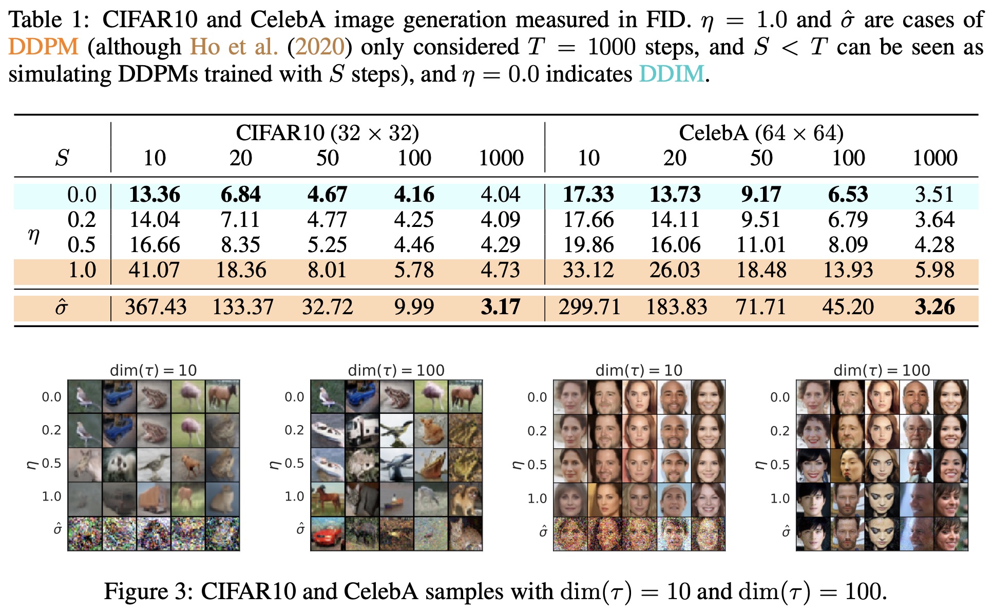
Experimental Results
The original paper compared different combinations of noise intensity and diffusion steps \dim(\boldsymbol{\tau}). The general result is that "the smaller the noise, the better the generation effect after acceleration," as shown below:
My reference implementation is as follows:
Github: https://github.com/bojone/Keras-DDPM/blob/main/ddim.py
My personal experimental conclusions are:
1. Contrary to intuition, the smaller the \sigma_t in the generation process, the relatively larger the noise and diversity of the final generated image;
2. The fewer the diffusion steps \dim(\boldsymbol{\tau}), the smoother the generated images, and the diversity also decreases;
3. Combining points 1 and 2, when the diffusion steps \dim(\boldsymbol{\tau}) decrease, \sigma_t can be appropriately reduced to keep the generated image quality roughly constant, which is consistent with the experimental conclusions of the original DDIM paper;
4. When \sigma_t is small, using fixed Sinusoidal encoding to represent t produces less noise in generated images compared to a trainable Embedding layer;
5. When \sigma_t is small, the U-Net architecture from the original paper (ddpm2.pyin Github) produces less noise than the U-Net architecture I designed (ddpm.pyin Github);
6. Overall, I feel that the generation effect of the noise-free process is not as good as the noisy process; without noise, the generation effect is heavily influenced by the model architecture.
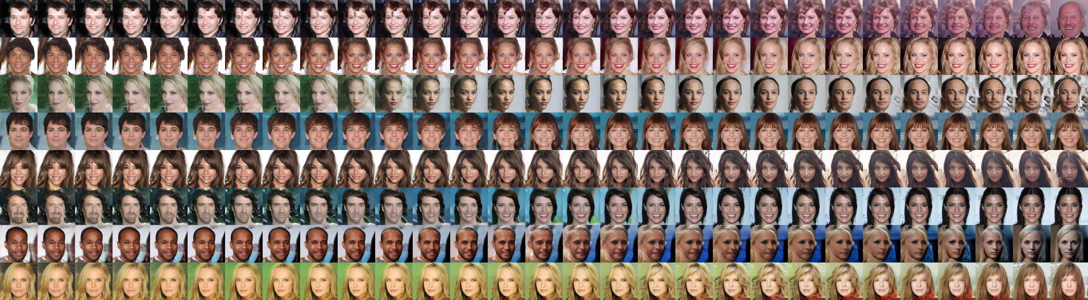
Furthermore, for DDIM with \sigma_t=0, it is a deterministic transformation that maps any normal noise vector to an image, which is almost identical to GANs. Thus, similar to GANs, we can interpolate between noise vectors and observe the corresponding generation effects. However, it should be noted that both DDPM and DDIM are sensitive to the noise distribution. Therefore, we cannot use linear interpolation but must use spherical interpolation (Slerp). Because of the additivity of normal distributions, if \boldsymbol{z}_1, \boldsymbol{z}_2 \sim \mathcal{N}(\boldsymbol{0}, \boldsymbol{I}), then \lambda\boldsymbol{z}_1 + (1-\lambda)\boldsymbol{z}_2 generally does not follow \mathcal{N}(\boldsymbol{0}, \boldsymbol{I}). Instead, we use: \boldsymbol{z} = \boldsymbol{z}_1 \cos\frac{\lambda\pi}{2} + \boldsymbol{z}_2 \sin\frac{\lambda\pi}{2}, \quad \lambda \in [0, 1]
Interpolation effect demonstration (model trained by myself):
Differential Equations
Finally, let’s focus on the case where \sigma_t = 0. At this point, Eq. [eq:sigma=0] can be equivalently rewritten as: \frac{\boldsymbol{x}_t}{\bar{\alpha}_t} - \frac{\boldsymbol{x}_{t-1}}{\bar{\alpha}_{t-1}} = \left(\frac{\bar{\beta}_t}{\bar{\alpha}_t} - \frac{\bar{\beta}_{t-1}}{\bar{\alpha}_{t-1}}\right) \boldsymbol{\epsilon}_{\boldsymbol{\theta}}(\boldsymbol{x}_t, t) When T is large enough, or when the difference between \alpha_t and \alpha_{t-1} is small enough, we can view the above equation as a finite difference form of some ordinary differential equation (ODE). Specifically, by introducing a virtual time parameter s, we get: \frac{d}{ds}\left(\frac{\boldsymbol{x}(s)}{\bar{\alpha}(s)}\right) = \boldsymbol{\epsilon}_{\boldsymbol{\theta}}\left(\boldsymbol{x}(s), t(s)\right)\frac{d}{ds}\left(\frac{\bar{\beta}(s)}{\bar{\alpha}(s)}\right) \label{eq:ode} Without loss of generality, assume s \in [0, 1], where s=0 corresponds to t=0 and s=1 corresponds to t=T. Note that the original DDIM paper directly used \frac{\bar{\beta}(s)}{\bar{\alpha}(s)} as the virtual time parameter, which is generally not ideal because its range is [0, \infty), and unbounded intervals are unfavorable for numerical solving.
Now, what we need to do is solve for \boldsymbol{x}(0) given \boldsymbol{x}(1) \sim \mathcal{N}(\boldsymbol{0}, \boldsymbol{I}). The iteration process of DDPM or DDIM corresponds to the Euler method for this ODE. It is well known that the Euler method is relatively the slowest in terms of efficiency. To accelerate the solution, one can use Heun’s method, Runge-Kutta methods, etc. In other words, by equating the generation process to solving an ODE, we can leverage numerical ODE solvers to provide more diverse means of accelerating the generation process.
Taking the default DDPM parameters T=1000, \alpha_t = \sqrt{1 - \frac{0.02t}{T}} as an example, we repeat the estimation made in "Generative Diffusion Models (Part 1): DDPM = Demolition + Construction": \log \bar{\alpha}_t = \sum_{k=1}^t \log\alpha_k = \frac{1}{2} \sum_{k=1}^t \log\left(1 - \frac{0.02k}{T}\right) < \frac{1}{2} \sum_{k=1}^t \left(- \frac{0.02k}{T}\right) = -\frac{0.005t(t+1)}{T} In fact, since each \alpha_k is very close to 1, the above estimation is a very good approximation. Since our starting point is p(\boldsymbol{x}_t|\boldsymbol{x}_0), we should start with \bar{\alpha}_t. Based on the above approximation, we can simply take: \bar{\alpha}_t = \exp\left(-\frac{0.005t^2}{T}\right) = \exp\left(-\frac{5t^2}{T^2}\right) If we take s=t/T as the parameter, then s \in [0, 1], and \bar{\alpha}(s) = e^{-5s^2}. Substituting this into Eq. [eq:ode] and simplifying, we get: \frac{d\boldsymbol{x}(s)}{ds} = 10s\left(\frac{\boldsymbol{\epsilon}_{\boldsymbol{\theta}}\left(\boldsymbol{x}(s), sT\right)}{\sqrt{1-e^{-10s^2}}} - \boldsymbol{x}(s)\right) We can also take s=t^2/T^2 as the parameter, in which case s \in [0, 1] and \bar{\alpha}(s) = e^{-5s}. Substituting this into Eq. [eq:ode] and simplifying, we get: \frac{d\boldsymbol{x}(s)}{ds} = 5\left(\frac{\boldsymbol{\epsilon}_{\boldsymbol{\theta}}\left(\boldsymbol{x}(s), \sqrt{s}T\right)}{\sqrt{1-e^{-10s}}} - \boldsymbol{x}(s)\right)
Summary
This article followed the derivation logic of the previous DDPM post to introduce DDIM. It re-examined the starting point of DDPM, removed p(\boldsymbol{x}_t|\boldsymbol{x}_{t-1}) from the derivation process, thereby obtaining a broader family of solutions and ideas for accelerating the generation process. Finally, this new family of solutions allows us to link the generation process with the solution of ordinary differential equations, enabling further research into the generation process using ODE methods.
Reprinting: Please include the original link: https://kexue.fm/archives/9181
More details on reprinting: Please refer to "Scientific Space FAQ".