Multi-task learning is a very broad topic, and the goals of multi-task learning vary in different scenarios. In "Talks on Multi-Task Learning (I): In the Name of Loss" and "Talks on Multi-Task Learning (II): Acting on Gradients", we understood the goal of multi-task learning as "doing every task well," specifically manifested as "treating every task as equally as possible," which we can call "Parallel Multi-Task Learning." However, not all multi-task learning goals are like this. In many scenarios, we primarily want to learn a specific main task, while the other tasks are merely auxiliary, hoping to improve the performance of the main task by adding the learning of other tasks. Such scenarios can be called "Primary-Secondary Multi-Task Learning."
In this context, if we continue to use the learning scheme of Parallel Multi-Task Learning—"doing every task well"—it might significantly degrade the performance of the main task. Therefore, this article continues along the idea of "acting on gradients" to explore training schemes for Primary-Secondary Multi-Task Learning.
Objective Form
In this article, we assume the reader has already read and basically understood the ideas and methods in "Talks on Multi-Task Learning (II): Acting on Gradients". From the gradient perspective, a necessary condition for keeping a certain loss function decreasing is that the update amount’s angle with its gradient must be at least greater than 90 degrees. This is the design philosophy throughout the text.
Constrained Optimization
Now assume that in a Primary-Secondary Multi-Task Learning scenario, we have n+1 loss functions for tasks, denoted as \mathcal{L}_0, \mathcal{L}_1, \dots, \mathcal{L}_n, where \mathcal{L}_0 is the primary task loss, which we want to be as small as possible. \mathcal{L}_1, \dots, \mathcal{L}_n are auxiliary losses, equivalent to regularization terms; we only hope they do not increase during the training process, but they do not necessarily need to "strive to become smaller."
Using the notation from the previous article, we denote the update amount at each step as \Delta\boldsymbol{\theta} = -\eta\boldsymbol{u}. Since we take \mathcal{L}_0 as the primary task, we naturally want to maximize the inner product of \boldsymbol{u} and \boldsymbol{g}_0. We can design the optimization objective as: \max_{\boldsymbol{u}} \langle\boldsymbol{u}, \boldsymbol{g}_0\rangle - \frac{1}{2}\Vert\boldsymbol{u}\Vert^2 Here \boldsymbol{g}_i = \nabla_{\boldsymbol{\theta}}\mathcal{L}_i is the gradient of the corresponding loss. Without other constraints, the solution would be \boldsymbol{u} = \boldsymbol{g}_0, which is ordinary gradient descent. However, we have auxiliary tasks \mathcal{L}_1, \dots, \mathcal{L}_n, and we hope they do not move in an increasing direction. So we must at least ensure \langle\boldsymbol{u}, \boldsymbol{g}_1\rangle \geq 0, \dots, \langle\boldsymbol{u}, \boldsymbol{g}_n\rangle \geq 0. These are the optimization constraints, making the total objective: \max_{\boldsymbol{u}} \langle\boldsymbol{u}, \boldsymbol{g}_0\rangle - \frac{1}{2}\Vert\boldsymbol{u}\Vert^2 \quad \text{s.t.} \,\, \langle\boldsymbol{u}, \boldsymbol{g}_1\rangle \geq 0, \dots, \langle\boldsymbol{u}, \boldsymbol{g}_n\rangle \geq 0 Solving this constrained optimization problem yields the update amount that satisfies the conditions.
Lagrange Multipliers
The standard scheme for solving such constrained optimization problems is the method of Lagrange multipliers, which integrates the constraints into the objective function, transforming it into a min-max problem: \max_{\boldsymbol{u}} \min_{\lambda_i \geq 0} \langle\boldsymbol{u}, \boldsymbol{g}_0\rangle - \frac{1}{2}\Vert\boldsymbol{u}\Vert^2 + \sum_i \lambda_i \langle\boldsymbol{u}, \boldsymbol{g}_i\rangle \label{eq:q-1}
Here, the summation over i is from 1 to n. How to understand this transformation? If \langle\boldsymbol{u}, \boldsymbol{g}_i\rangle > 0, then the \min_{\lambda_i \geq 0} step can only result in \lambda_i = 0, because only \lambda_i = 0 makes it minimal, at which point \lambda_i \langle\boldsymbol{u}, \boldsymbol{g}_i\rangle = 0. If \langle\boldsymbol{u}, \boldsymbol{g}_i\rangle = 0, then naturally \lambda_i \langle\boldsymbol{u}, \boldsymbol{g}_i\rangle = 0. If \langle\boldsymbol{u}, \boldsymbol{g}_i\rangle < 0, then the \min_{\lambda_i \geq 0} step would result in \lambda_i \to \infty, making \lambda_i \langle\boldsymbol{u}, \boldsymbol{g}_i\rangle \to -\infty. But remember, the optimization of \boldsymbol{u} is a \max operation, so between 0 and -\infty, it will naturally choose 0. That is, after completing this min-max optimization, it will automatically satisfy \langle\boldsymbol{u}, \boldsymbol{g}_i\rangle \geq 0 and \lambda_i \langle\boldsymbol{u}, \boldsymbol{g}_i\rangle = 0. This means the result of the min-max optimization is exactly equivalent to the original constrained max optimization.
To facilitate the subsequent derivation, we introduce notation similar to the previous article: \mathbb{Q}^n = \{(\lambda_1, \dots, \lambda_n) \mid \lambda_1, \dots, \lambda_n \geq 0\}, \quad \tilde{\boldsymbol{g}}(\lambda) = \sum_i \lambda_i \boldsymbol{g}_i Then equation [eq:q-1] can be written as: \max_{\boldsymbol{u}} \min_{\lambda \in \mathbb{Q}^n} \langle\boldsymbol{u}, \boldsymbol{g}_0 + \tilde{\boldsymbol{g}}(\lambda)\rangle - \frac{1}{2}\Vert\boldsymbol{u}\Vert^2 \label{eq:q-2}
Solving Algorithm
So far, we have transformed the solution for the update direction in Primary-Secondary Multi-Task Learning into a min-max problem [eq:q-2]. Next, similar to the method in the previous article, we first use the Minimax Theorem to swap the order of \max and \min, then further provide a solution method via the Frank-Wolfe algorithm, and finally compare the similarities and differences between this and the results of the previous article.
Swapping the Order
Note that the \max and \min in problem [eq:q-2] are ordered. Normally, the \min step must be completed before the \max step; swapping the order rashly might lead to incorrect results. However, the \min step is a constrained optimization, while the \max step is unconstrained, so the \max step is relatively simpler. If we can swap the order and perform the \max step first, the problem can be simplified.
Therefore, we first need to determine if the order of the two can be swapped. Fortunately, von Neumann proposed the beautiful Minimax Theorem. It tells us that if the feasible regions of the parameters for \min and \max are both convex sets, and the objective function is convex with respect to the \min parameters and concave with respect to the \max parameters, then the order of \min and \max can be swapped. Even more fortunately, it is easy to see that problem [eq:q-2] satisfies the conditions of the Minimax Theorem, so it is equivalent to: \min_{\lambda \in \mathbb{Q}^n} \max_{\boldsymbol{u}} \langle\boldsymbol{u}, \boldsymbol{g}_0 + \tilde{\boldsymbol{g}}(\lambda)\rangle - \frac{1}{2}\Vert\boldsymbol{u}\Vert^2 = \min_{\lambda \in \mathbb{Q}^n} \frac{1}{2}\Vert\boldsymbol{g}_0 + \tilde{\boldsymbol{g}}(\lambda)\Vert^2 \label{eq:q-3} Thus, we have simplified the problem to only a \min operation, where the right side of the equation is because the objective function on the left is just a quadratic function of \boldsymbol{u}, and its maximum is reached at \boldsymbol{u}^* = \boldsymbol{g}_0 + \tilde{\boldsymbol{g}}(\lambda). Substituting this gives the result on the right.
Simple Case
The problem has now become finding the weighted superposition of \boldsymbol{g}_0 and \boldsymbol{g}_1, \dots, \boldsymbol{g}_n with the minimum norm. As usual, let’s first try to solve the simplest case, which is n=1: \min_{\gamma \geq 0} \Vert\boldsymbol{g}_0 + \gamma\boldsymbol{g}_1\Vert^2. This has a clear geometric meaning and a simple analytical solution.
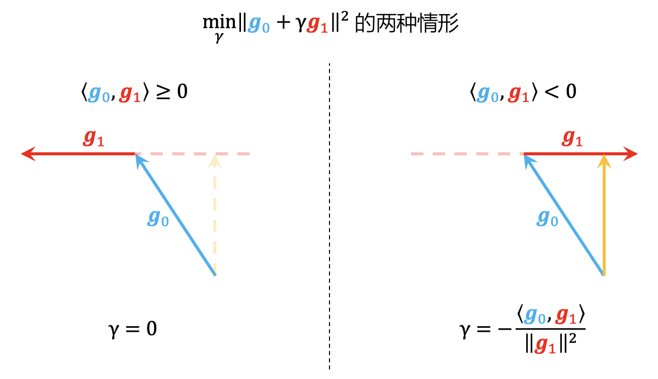
As shown in the figure above, there are two cases: the first case is \langle\boldsymbol{g}_0, \boldsymbol{g}_1\rangle \geq 0, which indicates that \boldsymbol{g}_0 and \boldsymbol{g}_1 are not in conflict, so we can just take \gamma = 0. The second case is \langle\boldsymbol{g}_0, \boldsymbol{g}_1\rangle < 0. As seen from the right figure above, the minimum value of \Vert\boldsymbol{g}_0 + \gamma\boldsymbol{g}_1\Vert^2 is reached when \boldsymbol{g}_0 + \gamma\boldsymbol{g}_1 is perpendicular to \boldsymbol{g}_1. Thus, solving \langle \boldsymbol{g}_0 + \gamma\boldsymbol{g}_1, \boldsymbol{g}_1\rangle = 0 yields \gamma = -\frac{\langle \boldsymbol{g}_0, \boldsymbol{g}_1\rangle}{\Vert\boldsymbol{g}_1\Vert^2}. Finally, when \Vert\boldsymbol{g}_1\Vert \neq 0, it can be written uniformly as: \gamma = \frac{\text{relu}(-\langle \boldsymbol{g}_0, \boldsymbol{g}_1\rangle)}{\Vert\boldsymbol{g}_1\Vert^2} \label{eq:gamma}
Iterative Solution
Next, we handle the general case, the idea of which still stems from the Frank-Wolfe algorithm.
First, we find the feasible direction e_{\tau} for the next update via \tau = \mathop{\text{argmin}}_i \langle \boldsymbol{g}_i, \boldsymbol{g}_0 + \tilde{\boldsymbol{g}}(\lambda^{(k)})\rangle. Then, we perform a one-dimensional search, but unlike before, this time we do not search by interpolating between \lambda^{(k)} and e_{\tau}. Instead, we directly re-determine the coefficient corresponding to \boldsymbol{g}_{\tau}. That is, we remove the \boldsymbol{g}_{\tau} part from \tilde{\boldsymbol{g}}(\lambda^{(k)}) and then re-calculate the coefficient for \boldsymbol{g}_{\tau} using the n=1 case algorithm.
From this, we obtain the following iterative process: \left\{\begin{aligned} &\tau = \mathop{\text{argmin}}_i \langle \boldsymbol{g}_i, \boldsymbol{g}_0+\tilde{\boldsymbol{g}}(\lambda^{(k)})\rangle\\ &\gamma = \mathop{\text{argmin}}_{\gamma} \left\Vert\boldsymbol{g}_0 + \tilde{\boldsymbol{g}}(\lambda^{(k)} - \lambda^{(k)}_{\tau} e_{\tau} + \gamma e_{\tau})\right\Vert^2 = \mathop{\text{argmin}}_{\gamma} \left\Vert\boldsymbol{g}_0 + \tilde{\boldsymbol{g}}(\lambda^{(k)}) - \lambda^{(k)}_{\tau}\boldsymbol{g}_{\tau} + \gamma \boldsymbol{g}_{\tau}\right\Vert^2\\ &\lambda^{(k+1)} = \lambda^{(k)} - \lambda^{(k)}_{\tau} e_{\tau} + \gamma e_{\tau} \end{aligned}\right.
Comparison
At this point, we have completed the solution for the Primary-Secondary Multi-Task Learning explored in this article. For students who have carefully derived the mathematical results of both articles, they will certainly feel that the methods and results of Parallel and Primary-Secondary types are very similar. Indeed, they have many similarities, but there are subtle differences.
To deepen everyone’s understanding, we can compare the similarities and differences between these two types of multi-task learning as follows:
| Parallel MTL (Previous) | Primary-Secondary MTL (This) | |
|---|---|---|
| Objective | Do every task well | Do main task well, don’t let auxiliary tasks worsen |
| Update Form | \Delta\boldsymbol{\theta} = -\eta\boldsymbol{u} | \Delta\boldsymbol{\theta} = -\eta\boldsymbol{u} |
| Math Definition | \max\limits_{\boldsymbol{u}}\min\limits_i \langle \boldsymbol{g}_i, \boldsymbol{u}\rangle - \frac{1}{2}\Vert \boldsymbol{u}\Vert^2 | \max\limits_{\boldsymbol{u}} \langle\boldsymbol{u},\boldsymbol{g}_0\rangle - \frac{1}{2}\Vert\boldsymbol{u}\Vert^2 s.t. \langle\boldsymbol{u},\boldsymbol{g}_1\rangle\geq 0,\dots,\langle\boldsymbol{u},\boldsymbol{g}_n\rangle\geq 0 |
| Dual Result | \min\limits_{\alpha\in\mathbb{P}^n} \Vert\tilde{\boldsymbol{g}}(\alpha)\Vert^2 | \min\limits_{\lambda\in\mathbb{Q}^n}\Vert\boldsymbol{g}_0 + \tilde{\boldsymbol{g}}(\lambda)\Vert^2 |
| Direction Vector | \boldsymbol{u}=\tilde{\boldsymbol{g}}(\alpha)=\sum\limits_i \alpha_i \boldsymbol{g}_i | \boldsymbol{u}=\boldsymbol{g}_0+\tilde{\boldsymbol{g}}(\lambda)=\boldsymbol{g}_0 + \sum\limits_i \lambda_i \boldsymbol{g}_i |
| Feasible Space | \mathbb{P}^n = \{(\alpha_1,\dots,\alpha_n) \mid \alpha_i\geq 0, \sum_i \alpha_i = 1\} | \mathbb{Q}^n=\{(\lambda_1,\dots,\lambda_n) \mid \lambda_i\geq 0\} |
| Iterative Steps | \left\{\begin{aligned} &\tau = \mathop{\text{argmin}}_i \langle \boldsymbol{g}_i, \tilde{\boldsymbol{g}}(\alpha^{(k)})\rangle\\ &\gamma = \mathop{\text{argmin}}_{\gamma} \Vert(1-\gamma)\tilde{\boldsymbol{g}}(\alpha^{(k)}) + \gamma \boldsymbol{g}_{\tau}\Vert^2\\ &\alpha^{(k+1)} = (1-\gamma)\alpha^{(k)} + \gamma e_{\tau} \end{aligned}\right. | \left\{\begin{aligned} &\tau = \mathop{\text{argmin}}_i \langle \boldsymbol{g}_i, \boldsymbol{g}_0+\tilde{\boldsymbol{g}}(\lambda^{(k)})\rangle\\ &\gamma = \mathop{\text{argmin}}_{\gamma} \Vert\boldsymbol{g}_0 + \tilde{\boldsymbol{g}}(\lambda^{(k)}) - \lambda^{(k)}_{\tau}\boldsymbol{g}_{\tau} + \gamma \boldsymbol{g}_{\tau}\Vert^2\\ &\lambda^{(k+1)} = \lambda^{(k)} - \lambda^{(k)}_{\tau} e_{\tau} + \gamma e_{\tau} \end{aligned}\right. |
After this comparison, it is not difficult to generalize the results to a hybrid multi-task learning with n primary tasks and m auxiliary tasks. Its dual result is: \min_{\alpha\in\mathbb{P}^n, \lambda\in\mathbb{Q}^m} \Vert\tilde{\boldsymbol{g}}(\alpha) + \tilde{\boldsymbol{g}}(\lambda)\Vert^2 As for the specific iterative algorithm, please think about it yourself!
Application Thoughts
In this section, we use a few examples to show that many common problems can correspond to this Primary-Secondary Multi-Task Learning. In a sense, Primary-Secondary MTL might be more common than Parallel MTL.
Regularization Loss
The most common example might be the regularization term added to the task loss function, such as L2 regularization: \mathcal{L}(\boldsymbol{\theta}) + \frac{\lambda}{2}\Vert\boldsymbol{\theta}\Vert^2 If we view \mathcal{L}(\boldsymbol{\theta}) and \frac{1}{2}\Vert\boldsymbol{\theta}\Vert^2 as losses for two tasks, this can also be seen as a multi-task learning problem. Obviously, we do not want \frac{1}{2}\Vert\boldsymbol{\theta}\Vert^2 to be as small as possible; we only hope that the addition of \frac{1}{2}\Vert\boldsymbol{\theta}\Vert^2 can improve the generalization performance of \mathcal{L}(\boldsymbol{\theta}). So this does not correspond to Parallel MTL but is closer to Primary-Secondary MTL.
The gradient of the L2 regularization term \frac{1}{2}\Vert\boldsymbol{\theta}\Vert^2 is simple: it is \boldsymbol{\theta}. Then, applying the result [eq:gamma] from this article, we can modify the optimizer to change the gradient term to: \boldsymbol{g} + \frac{\text{relu}(-\langle \boldsymbol{g}, \boldsymbol{\theta}\rangle)}{\Vert\boldsymbol{\theta}\Vert^2} In this way, we can add L2 regularization to the model without having to tune the regularization coefficient \lambda. Of course, one can also directly process the original update amount like AdamW to achieve a decoupled weight decay.
Besides this direct regularization of parameters, there are many other forms of auxiliary losses, such as adding contrastive learning losses to classification models, adding length penalties to generative models, etc. These practices more or less correspond to Primary-Secondary MTL, so one can try to apply the results of this article. If the calculation of the full gradient is too large, one can also use the approximation for the "shared encoder" case as in the previous article to reduce the computational cost.
Learning with Noisy Labels
Furthermore, there is a common training scenario that people might not realize is a multi-task learning problem, but it can essentially be understood as one: "Learning with Noisy Labels."
Suppose for the same task, we only have a small amount of accurately labeled clean data, but at the same time, we have a large amount of noisy data. Since there is more noisy data, we tend to learn primarily from the noisy data, assuming the corresponding loss is \mathcal{L}_0. However, due to the noise in the data, purely minimizing \mathcal{L}_0 might not yield an ideal model; it might memorize the incorrect labels. At this point, the clean data can come in handy. We can calculate a loss \mathcal{L}_1 using the clean data. Since the clean data has less noise, we can consider \mathcal{L}_1 to reflect the model’s true performance better than \mathcal{L}_0. Then we can add a constraint:
No matter how you minimize \mathcal{L}_0, you cannot let \mathcal{L}_1 increase. In other words, you can use noisy data for training, but you cannot let the performance on clean data worsen.
This is exactly a Primary-Secondary MTL problem with \mathcal{L}_0 as primary and \mathcal{L}_1 as auxiliary!
Coincidentally, a Google paper from last year, "Gradient-guided Loss Masking for Neural Machine Translation", also gave a similar approach, but with slightly different details. It calculates the gradient of each noisy sample with respect to the parameters and only keeps samples whose gradient has an angle of less than 90 degrees (inner product greater than 0) with the clean data gradient \nabla_{\boldsymbol{\theta}} \mathcal{L}_1. That is, everyone uses the inner product with the clean data gradient as the criterion. The difference is that in Primary-Secondary MTL, if the inner product is less than 0, a correction is made to the update amount, whereas in Google’s article, the corresponding samples are directly discarded.
Summary
This article extends the results of Parallel Multi-Task Learning from the previous article to "Primary-Secondary" Multi-Task Learning. That is, the goal of multi-task learning is no longer to do all tasks well, but to take one task as primary and the others as auxiliary. The results have many similarities with the original Parallel MTL, but the details are different. Finally, some classic examples of Primary-Secondary MTL, such as regularization terms and learning with noisy labels, were introduced.
Original Address: https://kexue.fm/archives/8907