Dropout is a classic approach to preventing overfitting, and many readers are likely already familiar with it. Interestingly, Dropout has recently seen something of a "renaissance," with several intriguing new applications emerging. Examples include SimCSE and R-Drop, which have sparked significant discussion. In particular, as noted in the article "Dropout Twice Again! This Time It Achieves SOTA on Supervised Tasks", we found that simple R-Drop can even rival adversarial training, which is quite surprising.
Generally, Dropout is applied to the output of each layer or to the model parameters; these are its two classic use cases. However, I recently learned about a novel application from the paper "Raise a Child in Large Language Model: Towards Effective and Generalizable Fine-tuning": applying it to the gradients.
Dropout on gradients? Most readers have probably never heard of this. So, how effective is it? Let’s take a closer look.
Methodology Overview
In short, this paper proposes an approach called "ChildTuning" to improve the performance of pre-trained models during fine-tuning. Here, "Child" refers to a "Children Network," meaning a sub-network selected from the pre-trained model for optimization. This helps mitigate the risk of overfitting associated with optimizing the entire model. The selection of the sub-network is divided into two methods: ChildTuning-D and ChildTuning-F.
ChildTuning-D
ChildTuning-D (Task-Dependent) is a task-specific selection method that requires training data from the downstream task for computation. Specifically, assume the training data is (x_1,y_1), (x_2,y_2), \dots, (x_n,y_n) and the model is p(y|x;\theta), where \theta represents all model parameters and \theta_i is the i-th parameter. We calculate the Fisher Information as a measure of parameter importance: F_i = \frac{1}{n}\sum_{j=1}^n \left(\frac{\partial \log p(y_j|x_j;\theta)}{\partial\theta_i}\right)^2 Once we have the importance metrics, we can rank each parameter and select the top-p most important ones (e.g., the top 20%, where p=0.2). During model updates, only these parameters are optimized. Since fewer parameters are being updated, the risk of overfitting is reduced. In practice, ChildTuning-D determines the parameters to be optimized before fine-tuning begins and keeps them fixed throughout the process.
It is important to note that parameter selection is done at the individual component level. This means that within a single parameter matrix, only a portion might be selected. Therefore, it’s not about skipping entire parameter matrices, but rather masking the corresponding gradients using a 0/1 matrix M. The update rule becomes g \leftarrow g \otimes M / p, where dividing by p maintains the overall scale of the updates. Parameters not selected have a gradient of 0 and thus are not updated. While this theoretically reduces the number of updated parameters, it does not save on computation; the authors position it strictly as a method to improve fine-tuning performance.
ChildTuning-F
ChildTuning-F (Task-Free) is a task-independent selection method, which can be more descriptively called "Gradient Dropout." While ChildTuning-D constructs a fixed 0/1 matrix M based on task data, ChildTuning-F constructs a random 0/1 matrix M at each update step, where the proportion of 1s is p, and modifies the gradient as g \otimes M / p. Essentially, this is applying Dropout to the gradients.
Note that even if a parameter’s current gradient is 0, it doesn’t necessarily mean the current update amount for that parameter is 0. This is because we typically use optimizers with momentum, such as SGDM or Adam. For these optimizers, the update amount is proportional to the momentum, which is a moving average of historical gradients: m_t = \beta m_{t-1} + (1-\beta)g_t. Thus, if the historical gradients were non-zero, the momentum (and the update) will likely remain non-zero even if the current gradient is 0.
I have a question here: according to the design philosophy of ChildTuning, the goal should be to select only a sub-network for updating at each step—meaning only a p proportion of parameters should be updated. However, based on the analysis above, applying Dropout to the gradients doesn’t strictly achieve this. To achieve that goal, one should apply Dropout to the update amount \Delta\theta itself. Yet, after repeatedly checking the original paper and its open-source code, I confirmed that the authors indeed mean applying Dropout to the gradients.
Experimental Results
According to the experimental results provided in the original paper, ChildTuning’s performance is quite impressive, showing improvements across almost all tasks, with the highest improvement reaching 8%.
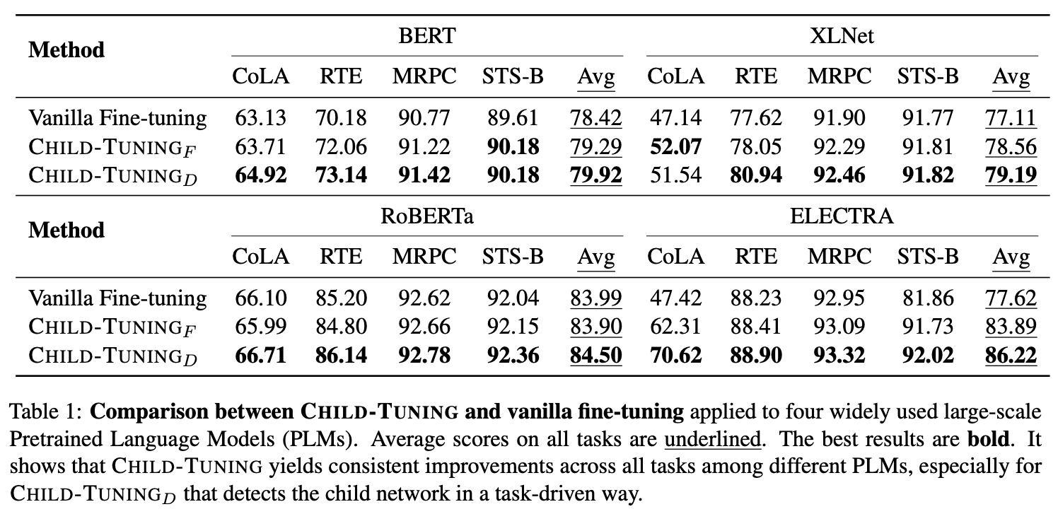
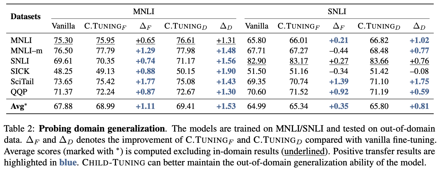
As seen from the tables, ChildTuning-D achieved improvements on almost all tasks, and ChildTuning-F was also effective on many. Furthermore, the paper describes results for the "large" versions of models. In private communication, the authors mentioned that the "base" versions also show improvements, though they were omitted due to space constraints.
Theoretical Reflections
ChildTuning-D ranks parameters based on Fisher Information, a concept with a long history. Its effectiveness is not surprising; similar works include "Training Neural Networks with Fixed Sparse Masks". Conversely, the fact that the task-independent ChildTuning-F (Gradient Dropout) is so effective warrants deeper thought.
Coincidentally, another paper from last year, "Regularizing Meta-Learning via Gradient Dropout", also applied Dropout to gradients. This suggests that Gradient Dropout can indeed be effective. But why?
The Paper’s Derivation
The original paper provides an explanation based on SGD, stating that Gradient Dropout increases the variance during the update process, which helps the model escape sub-optimal local minima.
Specifically, since we use SGD, the calculated gradient at each step has some randomness. Assume it follows a Gaussian distribution with mean \mu and variance \sigma^2. For ChildTuning-F, we introduce a random variable \varepsilon that is 1 with probability p and 0 with probability 1-p. Then we have: \begin{aligned} &\mathbb{E}[g\varepsilon/p]=\mathbb{E}[g]\mathbb{E}[\varepsilon]/p=\mu \\ &\mathbb{E}[(g\varepsilon/p)^2]=\mathbb{E}[g^2]\mathbb{E}[\varepsilon^2]/p^2 = (\mu^2+\sigma^2)/p \end{aligned} Therefore: \mathbb{V}ar[g\varepsilon/p] = \mathbb{E}[(g\varepsilon/p)^2] - \mathbb{E}[g\varepsilon/p]^2=\sigma^2 + \frac{1-p}{p}(\mu^2+\sigma^2) > \sigma^2 In other words, Gradient Dropout keeps the mean of the gradient unchanged but increases the variance. Since the update amount in SGD is proportional to the gradient, Gradient Dropout increases the variance of the updates. The paper argues this helps the model reach better convergence.
Missing the Point
This explanation seems reasonable and aligns with the intuition many people have—that stochastic gradient descent is better than full-batch gradient descent because of the noise. However, a bit of deeper thought reveals that this explanation is "missing the point."
The reason is simple: the analysis above applies to SGD, but in NLP, we almost always use Adam (or its variants). Does the conclusion hold for Adam? Unfortunately, no; in fact, the opposite happens. In Adam, in the long run, the update amount can be approximated as (\eta is the learning rate): \Delta\theta = \eta\frac{\mathbb{E}[g]}{\sqrt{\mathbb{E}[g^2]}} After adding Gradient Dropout, the update becomes: \eta\frac{\mathbb{E}[g\varepsilon/p]}{\sqrt{\mathbb{E}[(g\varepsilon/p)^2]}}=\eta\sqrt{p}\frac{\mathbb{E}[g]}{\sqrt{\mathbb{E}[g^2]}} As we can see, in the long run, adding Gradient Dropout to Adam is equivalent to reducing the learning rate to \sqrt{p} times its original value! Furthermore, because the learning rate (and thus the update amount) is reduced, the variance of the updates also decreases. That is to say, if you use the Adam optimizer, the actual situation is exactly the opposite of the paper’s explanation: the variance of the updates does not increase; it decreases.
The fundamental reason for this phenomenon is that when using an optimizer with moving averages, the update amount is no longer proportional to the gradient. Therefore, changes in the gradient do not necessarily correlate with changes in the update amount. This brings us back to my earlier question: why didn’t the authors simply apply Dropout to the update amount directly? If it were Update Dropout, the SGD-based derivation would carry over.
Personal Interpretation
However, I believe that even if the optimizer were restricted to SGD, or if Dropout were applied directly to the updates, the paper’s derivation wouldn’t fully explain its effectiveness. The reason is simple: there are many ways to achieve "constant mean, increased variance"—for example, adding Gaussian noise to the gradient. Would all such operations yield the same effect? I find it unlikely. I believe the explanation for Gradient Dropout or Update Dropout must lie in the sparsity they introduce.
On this issue, I am reminded of an article I wrote previously, "Optimization Algorithms from a Dynamical Perspective (VII): SGD \approx SVM?". That article suggests that the solutions found by SGD are essentially similar to SVM models: f_{\theta_T}(x) = \beta(x) + \sum_i \alpha_i (x) K(x, x_i) where x_i is the i-th training sample. What are its characteristics? K(x, x_i) acts like a "similarity function." This form implies that the model effectively "memorizes" the training set and, during prediction, retrieves information from the training set using K(x, x_i) as a similarity measure. Of course, this is a theoretical explanation; we don’t intentionally design models this way. We are simply observing that gradient descent is essentially memorizing samples and providing predictions in a manner similar to KNN. This makes it easy to understand why "more training data usually leads to better results."
Returning to ChildTuning-F, every time we sample a batch and apply Dropout to the gradients or updates, we can intuitively imagine—combined with the "memorization" explanation—that this is essentially "using only a small portion of parameters to memorize a small portion of samples," rather than using all parameters to memorize every small batch. This is similar to the idea of "not putting all your eggs in one basket." By distributing samples more evenly across parameters, the risk of overfitting is reduced.
Giving it a Try
For ChildTuning-F, if you know how to modify an optimizer, implementing either Gradient Dropout or Update Dropout is just one line of code. Therefore, it’s worth a try. What if it actually works?
I conducted tests on several CLUE tasks. The results are shown in the table below. The baseline code comes from "bert4keras in Hand, Baselines I Have: CLUE Benchmark Code". "grad drop" refers to Dropout on gradients, and "incre drop" refers to Dropout on the update amount. Green indicates an improvement over the baseline, while red indicates a decrease. Due to limited time and computing power, all results are from a single run and are subject to random fluctuations.
| IFLYTEK | TNEWS | AFQMC | OCNLI | CMNLI | WSC | CSL | |
|---|---|---|---|---|---|---|---|
| BERT | 60.06 | 56.80 | 72.41 | 73.93 | 79.56 | 78.62 | 83.93 |
| BERT-grad drop | 60.56 | 56.97 | 72.13 | 74.88 | 80.09 | 75.99 | 83.83 |
| BERT-incre drop | 59.99 | 56.78 | 72.66 | 74.51 | 79.36 | 77.30 | 84.20 |
| RoBERTa | 60.64 | 58.06 | 74.05 | 76.00 | 81.24 | 87.50 | 84.50 |
| RoBERTa-grad drop | 60.72 | 57.91 | 74.03 | 75.19 | 80.52 | 84.54 | 84.73 |
| RoBERTa-incre drop | 60.87 | 57.99 | 74.03 | 75.97 | 81.02 | 84.87 | 84.73 |
From the table, we can roughly observe:
Gradient Dropout and Update Dropout are generally comparable, with each having its own strengths and weaknesses.
The effect is more noticeable on BERT, while there is almost no effect on RoBERTa. This is consistent with the English experimental results provided in the paper.
This result is somewhat frustrating. It’s not that it’s ineffective, but normally, who would choose BERT over the better-performing RoBERTa if the speed is the same? If it doesn’t work well on RoBERTa, is it worth the effort? Of course, the paper reported the largest gains on Electra, which I haven’t tested. If any readers try it, please let me know the results.
Additionally, I didn’t have a particular interest in ChildTuning-D, and its implementation is slightly more complex, so I didn’t experiment with it. Readers who have tried it are welcome to share their feedback.
Summary
This article introduced the practice of adding Dropout to gradients to improve fine-tuning performance and provided a personal theoretical analysis. Overall, my feeling is: it’s worth a try and might be effective, but don’t set your expectations too high.
Original Address: https://kexue.fm/archives/8764