Currently, the mainstream implementation methods for WGAN include Weight Clipping, Spectral Normalization, and Gradient Penalty. This article introduces a new implementation scheme: Gradient Normalization. This scheme originates from two interesting papers: "Gradient Normalization for Generative Adversarial Networks" and "GraN-GAN: Piecewise Gradient Normalization for Generative Adversarial Networks".
What makes this interesting? As seen from the titles, these two papers appear to overlap significantly, suggesting they might be by the same author. However, they are actually from two different teams at roughly the same time—one published in ICCV and the other in WACV. They derived almost identical solutions based on the same assumptions. The degree of overlap is so high that I initially thought they were the same paper. Coincidences really are everywhere!
Background Review
We have introduced WGAN many times before, such as in "The Art of Mutual Confrontation: From Zero to WGAN-GP" and "From Wasserstein Distance and Duality Theory to WGAN", so I won’t repeat the details here. Simply put, the iterative form of WGAN is: \min_G \max_{\| D\|_{L}\leq 1} \mathbb{E}_{x\sim p(x)}\left[D(x)\right] - \mathbb{E}_{z\sim q(z)}\left[D(G(z))\right] The key here is that the discriminator D involves a constrained optimization problem, requiring the Lipschitz constraint \| D\|_{L}\leq 1 to be satisfied during the optimization process. Therefore, the difficulty of implementing WGAN lies in how to introduce this constraint into D.
To recap: if there exists a constant C such that for any x, y in the domain, |f(x)-f(y)|\leq C\| x - y\| holds, then we say f(x) satisfies the Lipschitz constraint (L-constraint). The minimum value of C is called the Lipschitz constant (L-constant), denoted as \| f\|_{L}. Thus, for the WGAN discriminator, two steps are required: 1. D must satisfy the L-constraint; 2. The L-constant must not exceed 1.
In fact, most current mainstream neural network models take the form of "linear combination + non-linear activation function." Since mainstream activation functions are "near-linear" (such as ReLU, LeakyReLU, SoftPlus, etc.) and the absolute values of their derivatives do not exceed 1, most current models actually satisfy the L-constraint. The key is ensuring the L-constant does not exceed 1. Of course, it doesn’t strictly have to be 1; it just needs to be bounded by some fixed constant.
Scheme Introduction
The ideas behind Weight Clipping and Spectral Normalization are similar: they both constrain the parameters to ensure the L-constant of each layer is bounded, thereby bounding the total L-constant. Gradient Penalty, on the other hand, notes that a sufficient condition for \| D\|_{L}\leq 1 is \|\nabla_x D(x)\| \leq 1, and imposes a "soft constraint" via the penalty term (\|\nabla_x D(x)\| - 1)^2.
The Gradient Normalization introduced here is based on the same sufficient condition. It uses the gradient to transform D(x) into \hat{D}(x) so that it automatically satisfies \|\nabla_x \hat{D}(x)\| \leq 1. Specifically, we usually use ReLU or LeakyReLU as activation functions. Under these activation functions, D(x) is actually a "piecewise linear function." This means that, except at the boundaries, D(x) is a linear function within local continuous regions. Correspondingly, \nabla_x D(x) is a constant vector.
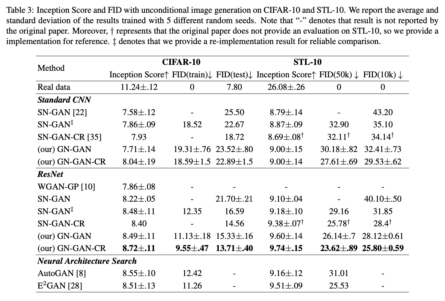
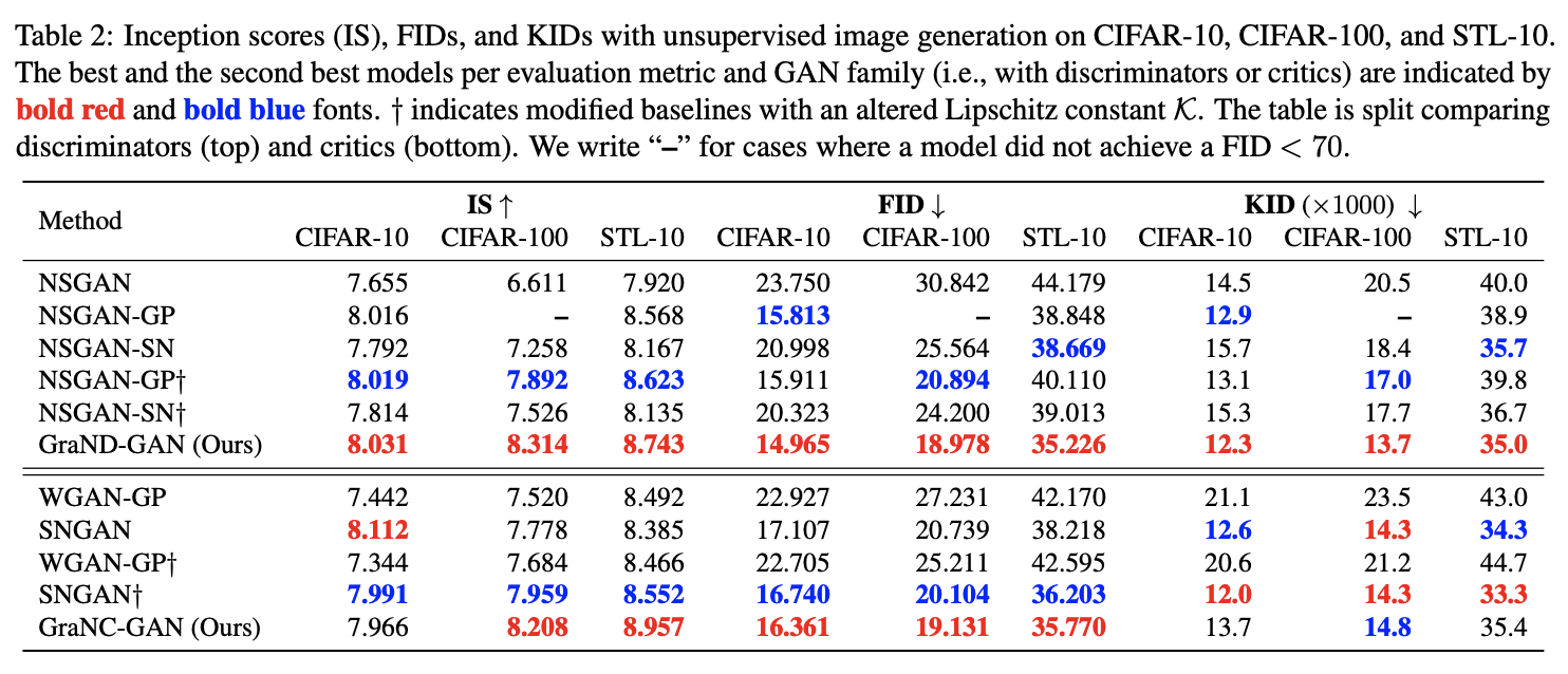
Thus, Gradient Normalization aims to set \hat{D}(x)=D(x)/\|\nabla_x D(x)\|. In this way: \|\nabla_x \hat{D}(x)\| = \left\| \nabla_x \left(\frac{D(x)}{\|\nabla_x D(x)\|}\right)\right\|=\left\| \frac{\nabla_x D(x)}{\|\nabla_x D(x)\|}\right\|=1 Of course, this might lead to division-by-zero errors, so the two papers proposed different solutions. The first paper (ICCV) directly added |D(x)| to the denominator, which also ensures the boundedness of the function: \hat{D}(x) = \frac{D(x)}{\|\nabla_x D(x)\| + |D(x)|} \in [-1,1] The second paper (WACV) more simply added an \epsilon: \hat{D}(x) = \frac{D(x)\cdot \|\nabla_x D(x)\|}{\|\nabla_x D(x)\|^2 + \epsilon} The second paper also mentioned testing \hat{D}(x)=D(x)/(\|\nabla_x D(x)\|+\epsilon), which yielded slightly worse but similar results.
Experimental Results
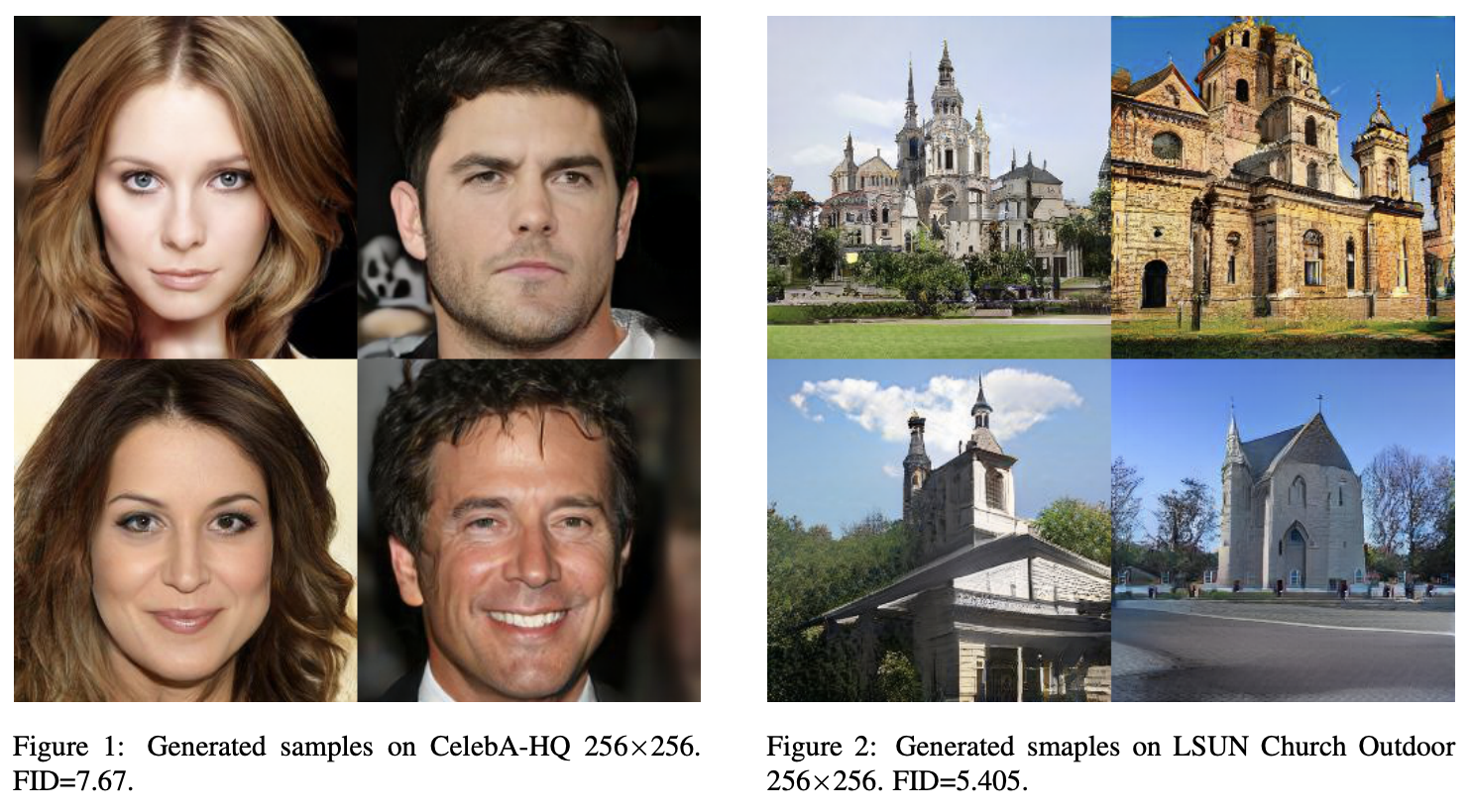
Let’s look at the experimental results. Naturally, since both were accepted into top conferences, the results are positive. Some results are shown below:
Remaining Doubts
The results look good, the theory seems sound, and it has been recognized by two top conferences, making it undoubtedly a good piece of work. However, my confusion is just beginning.
The most significant issue with this work is that, according to the piecewise linear function assumption, while the gradient of D(x) is locally constant, it is globally discontinuous (if the gradient were globally continuous and constant, it would be a linear function, not piecewise linear). However, D(x) itself is a continuous function. Thus, \hat{D}(x)=D(x)/\|\nabla_x D(x)\| is a continuous function divided by a discontinuous function, resulting in a discontinuous function!
So the question arises: it seems quite incredible that a discontinuous function can serve as a discriminator. This discontinuity is not just at a few boundary points; it exists between regions, making it a non-negligible presence. On Reddit, some readers had the same doubt, but the authors have not yet provided a reasonable explanation (Link).
Another issue is that if the piecewise linear assumption were truly valid, then using \hat{D}(x)=\left\langle \frac{\nabla_x D(x)}{\|\nabla_x D(x)\|}, x\right\rangle as a discriminator should theoretically be equivalent. However, my experimental results show that such a \hat{D}(x) performs extremely poorly. Therefore, one possibility is that Gradient Normalization is indeed effective, but the reason for its effectiveness is not as simple as the analysis in the two papers suggests; there may be more complex mechanisms at play. Furthermore, it’s possible that our understanding of GANs is still insufficient—that is, the requirements for the continuity of the discriminator might not be what we think.
Finally, in my experiments, the effect of Gradient Normalization was not as good as Gradient Penalty. Moreover, Gradient Penalty only requires second-order gradients when training the discriminator, whereas Gradient Normalization requires second-order gradients for training both the generator and the discriminator. Consequently, the speed of Gradient Normalization decreases significantly, and memory usage increases notably. From a personal practical experience standpoint, Gradient Normalization does not seem like a particularly friendly scheme.
Summary
This article introduced a new scheme for implementing WGAN—Gradient Normalization. The scheme is simple in form, and the reported results are quite good, but I believe there are still many questionable points within it.
Original Address: https://kexue.fm/archives/8757
For more details on reprinting, please refer to: "Scientific Space FAQ"