As the name suggests, this article introduces a post-processing trick for classification problems—CAN (Classification with Alternating Normalization), from the paper "When in Doubt: Improving Classification Performance with Alternating Normalization". Based on my practical tests, CAN does indeed improve the performance of multi-class classification problems in most cases, with almost no additional prediction cost, as it is merely a simple re-normalization operation on the prediction results.
Interestingly, the core idea of CAN is very intuitive—so intuitive that everyone has likely used similar reasoning in daily life. However, the CAN paper does not explain this intuition very clearly, presenting the method in a purely formal and experimental manner. In this post, I will try to explain the algorithmic idea as clearly as possible.
Conceptual Example
Suppose there is a binary classification problem. For input a, the model predicts p^{(a)} = [0.05, 0.95], so we predict class 1. Next, for input b, the model predicts p^{(b)} = [0.5, 0.5]. At this point, the model is in a state of maximum uncertainty, and we don’t know which class to output.
However, what if I tell you: 1. The class must be either 0 or 1; 2. The probability of each class occurring is 0.5. Given these two pieces of prior information, since the previous sample was predicted as class 1, based on a simple principle of balance, would we be more inclined to predict the second sample as class 0 to satisfy the second prior?
There are many such examples. For instance, if you are taking a 10-question multiple-choice test and you are confident in the first 9 answers, but have no idea about the 10th. If you notice that among the first 9 answers, A, B, and C have all appeared but D has not, would you be more inclined to guess D for the 10th question?
Behind these simple examples lies the same idea as CAN: it essentially uses the prior distribution to calibrate low-confidence predictions, making the distribution of the new predictions closer to the prior distribution.
Uncertainty
To be precise, CAN is a post-processing method targeting low-confidence predictions, so we first need a metric to measure the uncertainty of a prediction. A common measure is "Entropy" (refer to "Entropy" is not enough: From Entropy, Maximum Entropy Principle to Maximum Entropy Model (I)). For p=[p_1, p_2, \dots, p_m], it is defined as: H(p) = -\sum_{i=1}^m p_i \log p_i However, while entropy is a common choice, its results do not always align with our intuitive understanding. For example, for p^{(a)}=[0.5, 0.25, 0.25] and p^{(b)}=[0.5, 0.5, 0], applying the formula directly gives H(p^{(a)}) > H(p^{(b)}). But in our classification context, we would clearly consider p^{(b)} to be more uncertain than p^{(a)}, so using raw entropy is not entirely reasonable.
A simple correction is to calculate entropy using only the top-k probability values. Without loss of generality, assume p_1, p_2, \dots, p_k are the k highest probabilities, then: H_{\text{top-}k}(p) = -\sum_{i=1}^k \tilde{p}_i \log \tilde{p}_i where \tilde{p}_i = p_i \Big/ \sum_{i=1}^k p_i. To obtain a result in the range of 0 to 1, we take H_{\text{top-}k}(p) / \log k as the final uncertainty index.
Algorithm Steps
Now assume we have N samples to classify, and the model directly provides N probability distributions p^{(1)}, p^{(2)}, \dots, p^{(N)}. Assuming the test samples and training samples follow the same distribution, a perfect prediction should satisfy: \frac{1}{N} \sum_{i=1}^N p^{(i)} = \tilde{p} \label{eq:prior} where \tilde{p} is the prior distribution of the classes, which we can estimate directly from the training set. That is, the overall prediction results should be consistent with the prior distribution. However, due to model performance limitations, actual predictions may deviate significantly from this equation. At this point, we can manually correct this.
Specifically, we select a threshold \tau. Predictions with an index less than \tau are considered high-confidence, while those greater than or equal to \tau are low-confidence. Without loss of generality, assume the first n results p^{(1)}, p^{(2)}, \dots, p^{(n)} are high-confidence, and the remaining N-n are low-confidence. We consider the high-confidence part to be more reliable, so they are not corrected; instead, they are used as a "standard reference frame" to correct the low-confidence part.
Specifically, for each j \in \{n+1, n+2, \dots, N\}, we take p^{(j)} together with the high-confidence p^{(1)}, p^{(2)}, \dots, p^{(n)} and perform one "inter-row" normalization: p^{(k)} \leftarrow p^{(k)} \big/ \bar{p} \times \tilde{p}, \quad \bar{p} = \frac{1}{n+1} \left( p^{(j)} + \sum_{i=1}^n p^{(i)} \right) \label{eq:step-1} where k \in \{1, 2, \dots, n\} \cup \{j\}, and the multiplication and division are element-wise. It is easy to see that the purpose of this normalization is to make the average vector of all new p^{(k)} equal to the prior distribution \tilde{p}, thereby encouraging Equation [eq:prior] to hold. However, after this normalization, each p^{(k)} might no longer be normalized (sum to 1), so we must perform an "intra-row" normalization: p^{(k)}_i \leftarrow \frac{p^{(k)}_i}{\sum_{i=1}^m p^{(k)}_i} \label{eq:step-2} But then Equation [eq:prior] might no longer hold. Therefore, in theory, we can alternately iterate these two steps until convergence (though experimental results show that one iteration is usually best). Finally, we only keep the updated p^{(j)} as the prediction for the j-th sample, discarding the other p^{(k)}.
Note that this process must be executed for each low-confidence result j \in \{n+1, n+2, \dots, N\} individually. That is, corrections are performed sample by sample, not all at once. Each p^{(j)} is combined with the original high-confidence results p^{(1)}, p^{(2)}, \dots, p^{(n)} to iterate according to the steps above. Although p^{(1)}, p^{(2)}, \dots, p^{(n)} are updated during the iteration, those are only temporary results and are discarded; each new correction starts with the original p^{(1)}, p^{(2)}, \dots, p^{(n)}.
Reference Implementation
Here is the reference implementation code provided by the author:
# Prediction results, calculate accuracy before correction
y_pred = model.predict(
    valid_generator.fortest(), steps=len(valid_generator), verbose=True
)
y_true = np.array([d[1] for d in valid_data])
acc_original = np.mean([y_pred.argmax(1) == y_true])
print('original acc: %s' % acc_original)

# Evaluate uncertainty for each prediction
k = 3
y_pred_topk = np.sort(y_pred, axis=1)[:, -k:]
y_pred_topk /= y_pred_topk.sum(axis=1, keepdims=True)
y_pred_uncertainty = -(y_pred_topk * np.log(y_pred_topk)).sum(1) / np.log(k)

# Select threshold, split into high and low confidence parts
threshold = 0.9
y_pred_confident = y_pred[y_pred_uncertainty < threshold]
y_pred_unconfident = y_pred[y_pred_uncertainty >= threshold]
y_true_confident = y_true[y_pred_uncertainty < threshold]
y_true_unconfident = y_true[y_pred_uncertainty >= threshold]

# Display accuracy for both parts
# Generally, high-confidence accuracy is much higher than low-confidence
acc_confident = (y_pred_confident.argmax(1) == y_true_confident).mean()
acc_unconfident = (y_pred_unconfident.argmax(1) == y_true_unconfident).mean()
print('confident acc: %s' % acc_confident)
print('unconfident acc: %s' % acc_unconfident)

# Estimate prior distribution from the training set
prior = np.zeros(num_classes)
for d in train_data:
    prior[d[1]] += 1.

prior /= prior.sum()

# Correct low-confidence samples one by one and re-evaluate accuracy
right, alpha, iters = 0, 1, 1
for i, y in enumerate(y_pred_unconfident):
    Y = np.concatenate([y_pred_confident, y[None]], axis=0)
    for j in range(iters):
        Y = Y**alpha
        Y /= Y.mean(axis=0, keepdims=True)
        Y *= prior[None]
        Y /= Y.sum(axis=1, keepdims=True)
    y = Y[-1]
    if y.argmax() == y_true_unconfident[i]:
        right += 1

# Output final accuracy after correction
acc_final = (acc_confident * len(y_pred_confident) + right) / len(y_pred)
print('new unconfident acc: %s' % (right / (i + 1.)))
print('final acc: %s' % acc_final)
Experimental Results
So, how much improvement can such a simple post-processing step bring? The experimental results given in the original paper are quite impressive:
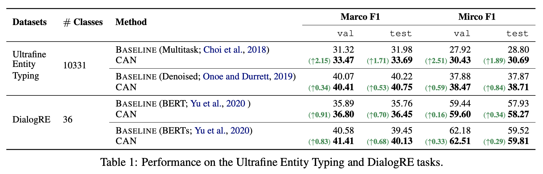
I also conducted experiments on two Chinese text classification tasks from CLUE, which showed some improvement, though not as dramatic (validation set results):
| IFLYTEK (119 classes) | TNEWS (15 classes) | |
|---|---|---|
| BERT | 60.06% | 56.80% |
| BERT + CAN | 60.52% | 56.86% |
| RoBERTa | 60.64% | 58.06% |
| RoBERTa + CAN | 60.95% | 58.00% |
Generally speaking, the more classes there are, the more significant the performance improvement. If the number of classes is small, the improvement might be slight or even result in a minor decrease (though any decrease is usually negligible). Thus, this can be considered an "almost free lunch." Regarding hyperparameter selection, for the Chinese results above, I used only 1 iteration, k=3, and \tau=0.9. After simple tuning, this combination was found to be quite optimal.
Some readers might wonder if the assumption that "high-confidence results are more reliable" actually holds. In my two Chinese experiments, it clearly does. For example, in the IFLYTEK task, the accuracy of the filtered high-confidence set was 0.63+, while the low-confidence set was only 0.22+. Similarly, for TNEWS, the high-confidence set accuracy was 0.58+, while the low-confidence set was 0.23+.
Personal Evaluation
Finally, let’s reflect on and evaluate CAN more comprehensively.
First, a natural question is why we don’t just correct all low-confidence results together with the high-confidence ones in a single batch, rather than correcting them one by one. I don’t know if the original authors compared this, but I did test this idea. The result was that batch correction sometimes matched per-sample correction but sometimes performed worse. This makes sense: the intent of CAN is to use the prior distribution and high-confidence results to correct low-confidence ones. In this process, the more low-confidence results you include, the larger the potential bias. Therefore, in theory, per-sample correction is more reliable than batch correction.
Regarding the original paper, readers who have read it might notice three main differences between this introduction and the original text:
1. Different calculation of the uncertainty index. According to the original paper, the uncertainty index is calculated as: -\frac{1}{\log m} \sum_{i=1}^k p_i \log p_i That is, it also uses the entropy of the top-k probabilities, but it does not re-normalize these k probabilities, and the factor used to compress the result into the 0–1 range is \log m instead of \log k (since it isn’t re-normalized, only dividing by \log m ensures the result stays between 0 and 1). In my tests, this method often results in values significantly smaller than 1, which makes it harder to perceive and tune the threshold.
2. Different presentation style. The original paper presents the CAN algorithm in a purely mathematical and matrix-oriented way, without explaining the underlying intuition. This is quite unfriendly for understanding. If readers do not think deeply about the principles themselves, it is hard to understand why such a post-processing method would improve classification, and once understood, it might feel somewhat over-complicated.
3. Slight difference in the algorithm flow. The original paper introduces a parameter \alpha during the iteration, changing Equation [eq:step-1] to: p^{(k)} \leftarrow [p^{(k)}]^{\alpha} \big/ \bar{p} \times \tilde{p}, \quad \bar{p} = \frac{1}{n+1} \left( [p^{(j)}]^{\alpha} + \sum_{i=1}^n [p^{(i)}]^{\alpha} \right) That is, each result is raised to the power of \alpha before iterating. The original paper does not explain this, and in my view, this parameter is purely for hyperparameter tuning (with more parameters, you can always find a way to show improvement) and lacks much practical significance. Furthermore, in my experiments, \alpha=1 was basically the optimal choice, and fine-tuning \alpha rarely yielded substantial gains.
Summary
This article introduced a simple post-processing trick called CAN, which leverages the prior distribution to re-normalize prediction results, improving classification performance with almost no added computational cost. Based on my experiments, CAN does provide a boost to classification effects, and generally, the more classes involved, the more obvious the improvement.
Original address: https://kexue.fm/archives/8728. Please include this link when reposting.
For more details on reposting, please refer to: Scientific Space FAQ.