In machine learning, we often encounter non-smooth functions. However, our optimization methods are typically gradient-based, which means that smooth models are generally more conducive to optimization (as their gradients are continuous). Consequently, there is a need to find smooth approximations for non-smooth functions. In fact, this blog has discussed related topics several times, such as “Seeking a Smooth Maximum Function” and “Miscellaneous Talk on Function Smoothing: Differentiable Approximations of Non-differentiable Functions”. However, previous discussions lacked a certain level of methodological generality.
Recently, I learned a relatively universal approach from the paper “SAU: Smooth activation function using convolution with approximate identities”: using the Dirac delta function to construct smooth approximations. How universal is it? Theoretically, any function with a countable number of discontinuities can be used to construct a smooth approximation using this method! Personally, I find this quite interesting.
The Dirac Delta Function
In a much earlier article, “The Eerie Dirac Function”, we introduced the Dirac delta function. In modern mathematics, the Dirac delta function is defined as a “functional” rather than a “function,” but for most readers, it is easier to accept it by treating it as a function.
Simply put, the Dirac delta function \delta(x) satisfies:
1. \forall x \neq 0, \delta(x) = 0;
2. \delta(0) = \infty;
3. \int_{-\infty}^{\infty} \delta(x) dx = 1.
Intuitively, \delta(x) can be viewed as a continuous probability density function with a sample space of all real numbers \mathbb{R}, but where the probability is non-zero only at x=0. That is, it has a mean of 0 and a variance of 0. Therefore, any sample taken from it must be 0. Consequently, the following identity holds: \int_{-\infty}^{\infty} f(x)\delta(x) dx = f(0) Or: \int_{-\infty}^{\infty} f(y)\delta(x-y) dy = f(x) \label{eq:base} This is arguably the most important property of the Dirac delta function and is the primary identity we will use later.
Smooth Approximation
If we can find a smooth approximation of \delta(x), denoted as \varphi(x) \approx \delta(x), then according to equation [eq:base], we have: g(x) = \int_{-\infty}^{\infty} f(y)\varphi(x-y) dy \approx f(x) Since \varphi(x) is smooth, g(x) is also smooth. This means that g(x) is a smooth approximation of f(x)! This is the core idea of constructing a smooth approximation of f(x) with the help of a smooth approximation of the Dirac delta function. In this process, there are few restrictions on the form and continuity of f(x); for example, f(x) is allowed to have a countable number of discontinuities (such as the floor function [x]).
So, what are the smooth approximations of the Dirac delta function? There are several well-known ones, such as: \delta(x) = \lim_{\sigma\to 0} \frac{e^{-x^2/2\sigma^2}}{\sqrt{2\pi}\sigma} \label{eq:g} Or: \delta(x) = \frac{1}{\pi} \lim_{a \to 0}\frac{a}{x^2+a^2} Simply put, the goal is to find a non-negative function with a bell-shaped curve like the normal distribution and find a way to make the width of the bell gradually approach 0 while maintaining an integral of 1. Another approach is to note that: \int_{-\infty}^x \delta(t)dt = \theta(x) = \left\{\begin{aligned}1,\,\, (x > 0) \\ 0,\,\, (x < 0)\end{aligned}\right. That is, the integral of the Dirac delta function is the “unit step function” \theta(x). If we can find a smooth approximation of \theta(x), then its derivative will be a smooth approximation of the Dirac delta function. Smooth approximations of \theta(x) are the so-called “S-shaped” curves, such as the sigmoid function \sigma(x)=1/(1+e^{-x}). Thus, we have: \delta(x) = \lim_{t\to \infty} \frac{d}{dx}\sigma(tx) = \lim_{t\to \infty} \frac{e^{tx}t}{(1+e^{tx})^2} \label{eq:s} Equations [eq:g] and [eq:s] are the two most commonly used approximations.
ReLU Activation
Now, using the above logic as a tool, let us derive various smooth approximations of the ReLU activation function \max(x,0).
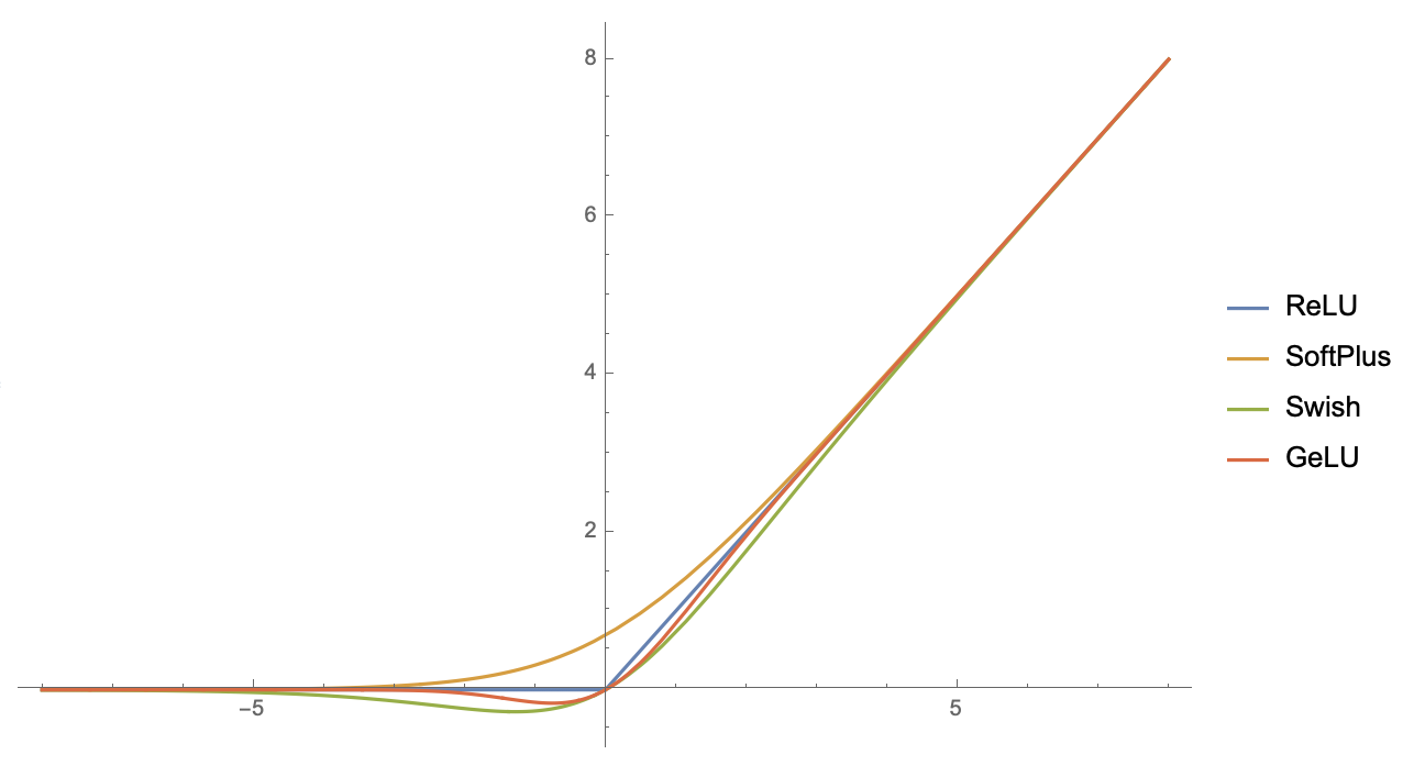
For instance, using equation [eq:s], we get: \begin{aligned} \max(x,0) \approx&\, \int_{-\infty}^{\infty} \frac{e^{t(x-y)}t}{(1+e^{t(x-y)})^2} \max(y,0) dy\\ =&\, \int_0^{\infty} \frac{e^{t(x-y)}ty}{(1+e^{t(x-y)})^2}dy = \frac{\log(1+e^{tx})}{t} \end{aligned} When t=1, this is the SoftPlus activation function.
If we use equation [eq:g] instead, the result is: \begin{aligned} \max(x,0) \approx&\, \int_{-\infty}^{\infty} \frac{e^{-(x-y)^2/2\sigma^2}}{\sqrt{2\pi}\sigma} \max(y,0) dy\\ =&\, \int_0^{\infty} \frac{e^{-(x-y)^2/2\sigma^2} y}{\sqrt{2\pi}\sigma}dy\\ =&\, \frac{1}{2} \left[x \,\text{erf}\left(\frac{x}{\sqrt{2} \sigma}\right)+x+\sqrt{\frac{2}{\pi }} \sigma e^{-\frac{x^2}{2 \sigma^2}}\right] \end{aligned} This smooth approximation of ReLU does not seem to have been widely studied.
Of course, if we only want a smooth approximation of the ReLU function, there are simpler ways. For example, noting that \max(x,0)=x\theta(x), where \theta(x) is the unit step function mentioned earlier, the problem transforms into finding a smooth approximation for \theta(x). We already know that the sigmoid is one such approximation, so we quickly obtain: \max(x,0) \approx x\sigma(tx) When t=1, this is the Swish activation function. If we use equation [eq:g] for the calculation, we get: \begin{aligned} \max(x,0) \approx&\, x\int_{-\infty}^{\infty} \frac{e^{-(x-y)^2/2\sigma^2}}{\sqrt{2\pi}\sigma} \theta(y) dy\\ =&\, x\int_0^{\infty} \frac{e^{-(x-y)^2/2\sigma^2}}{\sqrt{2\pi}\sigma}dy = \frac{1}{2}\left[x + x\,\text{erf}\left(\frac{x}{\sqrt{2}\sigma}\right)\right] \end{aligned} When \sigma=1, this is the GeLU activation function.
Integer Function
Readers might feel this is not yet impressive enough, as the derivations above resulted in existing functions that could be derived without the Dirac delta function. Now, let us add a non-trivial example: a smooth approximation of the integer function.
Integer functions include the ceiling and floor functions. They differ in definition but are not fundamentally different. Here, we take the floor function as an example, denoted as: = n, \,\,\text{if and only if there exists } n \in \mathbb{Z} \text{ such that } x \in [n, n + 1)
Suppose \varphi(x) is a smooth approximation of the Dirac delta function. Then: \approx \int_{-\infty}^{\infty} \varphi(x-y)[y]dy = \sum_{n=-\infty}^{\infty}n\int_n^{n+1} \varphi(x-y)dy Let \Phi(x) be the antiderivative of \varphi(x). Then the antiderivative of \varphi(x-y) with respect to y is -\Phi(x-y). Thus: \begin{aligned} [x] \approx&\, \sum_{n=-\infty}^{\infty}n\big[\Phi(x-n) - \Phi(x-n-1)\big]\\ =&\, \lim_{M,N\to\infty}\sum_{n=-M}^{N}(n-1)\Phi(x-n) - n\Phi(x-n-1) + \Phi(x-n)\\ =&\, \lim_{M,N\to\infty} -N\Phi(x-N-1) - (M+1)\Phi(x+M) + \sum_{n=-M}^{N} \Phi(x-n) \end{aligned} For \Phi(x), we have \Phi(-\infty)=0 and \Phi(\infty)=1. Assuming the range of interest satisfies -M \ll x \ll N, then \Phi(x-N-1) \approx 0 and \Phi(x+M) \approx 1. Thus, at this point: \begin{aligned} [x] \approx&\, -M-1 + \sum_{n=-M}^{N} \Phi(x-n)\\ =&\, \sum_{n=-M}^0 \big[\Phi(x-n)-1\big] + \sum_{n=1}^N \Phi(x-n) \end{aligned} Using \Phi(x)=\sigma(tx) as an example, with t=10, M=5, N=10, the result is as follows:
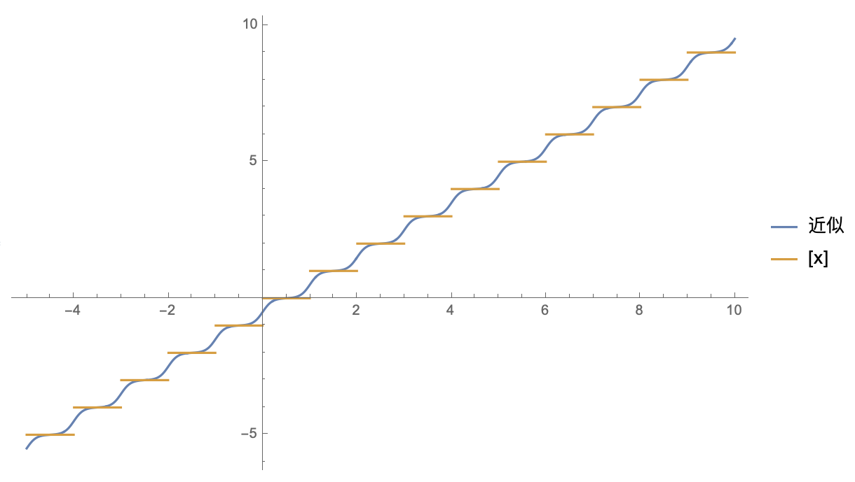
As we can see, it is indeed very close to [x]. Increasing t can further improve the degree of approximation.
Summary
This article introduced a method for constructing smooth approximations using the Dirac delta function. Its characteristic is its generality, as it does not impose strict requirements on the original function. As examples, we used it to derive various common approximations of the ReLU function and a smooth approximation of the floor function.
When reposting, please include the original address of this article: https://kexue.fm/archives/8718
For more detailed reposting matters, please refer to: “Scientific Space FAQ”