Since SimCLR made a splash in unsupervised visual learning, contrastive learning has become increasingly popular in CV and even NLP, leading to a surge in related research and applications. A well-known drawback of standard contrastive learning is its requirement for a large batch size (SimCLR performs best at batch_size=4096); performance drops significantly when the batch size is small. Consequently, one direction for improvement in subsequent work has been to reduce this dependency on large batch sizes. This leads to a natural question: What exactly is the reason why standard contrastive learning performs poorly with small batch sizes?
Recently, a paper titled "Simpler, Faster, Stronger: Breaking The log-K Curse On Contrastive Learners With FlatNCE" provided an answer to this question: floating-point error. It sounds almost unbelievable, but the paper’s analysis is quite reasonable, and the proposed improvement, FlatNCE, indeed works better, making it quite convincing.
The Subtle Details
Next, I will introduce the main content of the original paper using my own understanding and notation. I won’t review Contrastive Learning in detail here. Generally speaking, for a given sample x, we need to construct K paired samples y_1, y_2, \dots, y_K, where y_t is the positive sample and the rest are negative samples. We then score each sample pair (x, y_i), denoted as s_1, s_2, \dots, s_K. Contrastive learning aims to widen the score gap between positive and negative pairs, usually using cross-entropy as the loss: -\log \frac{e^{s_t}}{\sum\limits_i e^{s_i}} = \log \left(\sum_i e^{s_i}\right) - s_t = \log \left(1 + \sum_{i\neq t} e^{s_i - s_t}\right) For simplicity, let \xi = \sum_{i\neq t} e^{s_i - s_t}. In practice, positive samples are usually high-similarity samples generated via data augmentation, while negative samples are all other samples within the batch. Thus, negative samples can roughly be considered as K-1 randomly selected samples. This implies that the gap between positive and negative pairs is quite distinct, making it easy for the model to achieve s_t \gg s_i (i \neq t), i.e., e^{s_i - s_t} \approx 0. Consequently, when the batch size is small (equivalent to K being small), \xi will be very close to 0, meaning the loss function above will also be very close to 0.
A loss function close to 0 usually implies that the gradient is also close to 0. However, this does not mean the model’s update magnitude is small. Because current contrastive learning methods use adaptive optimizers like Adam, their update magnitude roughly takes the form \frac{\text{gradient}}{\sqrt{\text{gradient} \otimes \text{gradient}}} \times \text{learning rate}. This means that no matter how small the gradient is, as long as it is stable, the update magnitude will remain at the order of the learning rate. Contrastive learning fits this scenario. To make e^{s_i - s_t} \to 0, one needs s_i - s_t \to -\infty. However, scores in contrastive learning are typically cosine similarities divided by a temperature parameter, so they are bounded; s_i - s_t \to -\infty is unachievable. Therefore, after a certain number of training steps, the loss function will remain close to 0 but greater than 0 for a long time.
However, the calculation of \xi itself involves floating-point errors. When \xi is very close to 0, the floating-point error might be larger than the exact value. Then, the calculation of \log(1+\xi) also involves floating-point errors, and subsequently, the calculation of the gradient does as well. This series of accumulated errors likely results in the final calculated gradient being close to random noise, failing to provide effective guidance for updates. This is what the original paper identifies as the reason why contrastive learning performance degrades significantly at small batch sizes.
From Subtle to Significant
Once this reason is understood, it is not difficult to propose a targeted solution. By taking the first-order expansion of the loss function, we have: \log \left(1 + \sum_{i\neq t} e^{s_i - s_t}\right) \approx \sum_{i\neq t} e^{s_i - s_t} In other words, after a certain number of training steps, the model effectively uses \xi as the loss function. Of course, since \log(1+\xi) \leq \xi (i.e., \xi is an upper bound for \log(1+\xi)), even if we used \xi as the loss function from the start, the result wouldn’t differ much. The main issue now is solving the floating-point error problem caused by \xi being too close to 0. As mentioned, the update magnitude of adaptive optimizers is roughly \frac{\text{gradient}}{\sqrt{\text{gradient} \otimes \text{gradient}}} \times \text{learning rate}. This means if we directly multiply the loss function by a constant, the update magnitude theoretically remains unchanged. Since \xi is too small, we can simply multiply it by a constant to scale it up.
What should we multiply it by? A straightforward idea is that the loss function should neither be too small nor too large; keeping it at the \mathcal{O}(1) level is best. So, we might as well multiply it by the reciprocal of \xi, using: \frac{\xi}{\text{sg}(\xi)} = \frac{\sum\limits_{i\neq t} e^{s_i - s_t}}{\text{sg}\left(\sum\limits_{i\neq t} e^{s_i - s_t}\right)} \label{eq:flatnce-1} as the loss function. Here, \text{sg} stands for stop_gradient (referred to as "detach" in the original paper), meaning the denominator is treated purely as a constant, and the gradient is only calculated for the numerator. This is the alternative proposed by the original paper, called FlatNCE.
However, the loss function form with the \text{sg} operator is not what we are used to. We can transform it. Observing that: \nabla_{\theta}\left(\frac{\xi}{\text{sg}(\xi)}\right) = \frac{\nabla_{\theta}\xi}{\xi} = \nabla_{\theta}\log \xi In other words, the gradient provided by \frac{\xi}{\text{sg}(\xi)} as a loss function is identical to the gradient of \log \xi. Therefore, we can replace the loss function with \log \xi without the \text{sg} operator: \log\left(\sum\limits_{i\neq t} e^{s_i - s_t}\right) = \log\left(\sum\limits_{i\neq t} e^{s_i}\right) - s_t \label{eq:flatnce-2} Compared to cross-entropy, the above loss simply removes the positive pair score s_t from the \text{logsumexp} operation. Note that \text{logsumexp} can usually be calculated efficiently without floating-point errors dominating. Thus, using the above loss function to replace cross-entropy is theoretically equivalent to cross-entropy but practically performs better at small batch sizes. Additionally, it should be noted that the result of the above equation is not necessarily non-negative, so encountering negative loss values during training is normal and not unexpected.
Practical Insights
The analysis seems to make sense, but is it actually effective? Naturally, we must look at the experiments. Unsurprisingly, FlatNCE works very well.
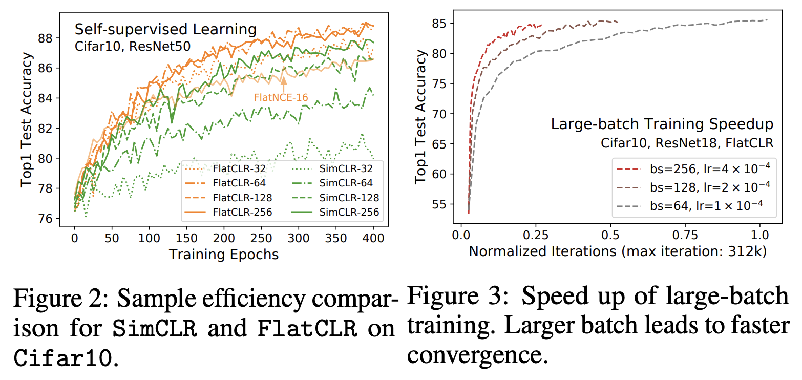
The experiments in the original paper are focused on CV, primarily replacing the SimCLR loss with FlatNCE. The corresponding results are called FlatCLR. What we care about most is whether FlatNCE truly solves the dependency on large batch sizes. The following image provides an affirmative answer:
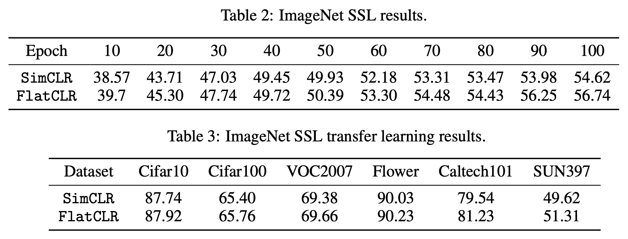
Below is a comparison of SimCLR and FlatCLR across various tasks, demonstrating the superior performance of FlatCLR:
Critical Reflections
Overall, the results of the original paper are highly creative. The perspective of "floating-point error" is very unique yet precise, deserving praise.
Intuitively, the original goal of cross-entropy is to make the "difference between positive and negative scores as large as possible." This is fine for regular classification problems, but it is insufficient for contrastive learning. Because the purpose of contrastive learning is to learn features, in addition to the "coarse" feature of the positive sample scoring higher than negative samples, negative samples must continue to be compared against each other to learn finer features. The goal of FlatNCE is to make "positive scores as large as possible and negative scores as small as possible." That is, it shifts from learning relative values to learning absolute values, allowing optimization to continue even after positive and negative samples are separated by a certain distance, rather than stopping prematurely (for non-adaptive optimizers) or letting noise from floating-point errors dominate (for adaptive optimizers).
However, some aspects of the original paper’s presentation are worth critiquing. For instance, the paper spends a significant amount of space discussing Mutual Information (MI) estimation, which has no substantial connection to the main thesis and increases the difficulty for the reader. Of course, a paper is different from a popular science article; adding extra theoretical derivations to make the article more substantial is understandable, though it would have been better to highlight the floating-point error analysis more prominently. Furthermore, the part I find most difficult to understand is why the paper presents Eq. [eq:flatnce-1] as the final result. This "stop_gradient" notation, while not difficult, is not user-friendly. Usually, this method is only used as a last resort when a primitive function cannot be found, but that is clearly not the case for FlatNCE.
Summary
This article introduced a new work in contrastive learning that analyzes the floating-point error problem of cross-entropy during small-batch training. It points out that this might be the primary reason for the poor performance of small-batch contrastive learning and proposes an improved loss function, FlatNCE. Experiments show that contrastive learning based on FlatNCE can indeed alleviate the dependency on large batch sizes and achieve better results.
When reposting, please include the original address of this article: https://kexue.fm/archives/8586
For more detailed reposting matters, please refer to: "Scientific Space FAQ"