Orthogonal Matrix Transforming One Unit Vector to Another

Two-Dimensional Case

It is not difficult to imagine that this is essentially a vector transformation problem (such as rotation or reflection) within the two-dimensional sub-plane formed by \boldsymbol{a} and \boldsymbol{b}. Therefore, let us first consider the case where d=2.

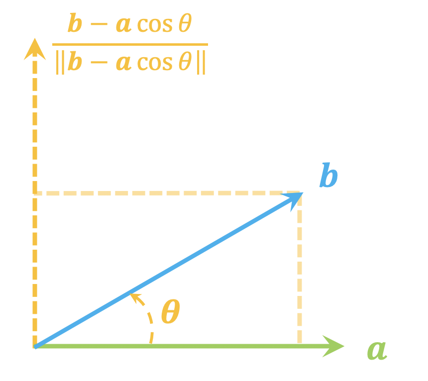
As shown in the figure above, through orthogonal decomposition, we can obtain a vector \boldsymbol{b} - \boldsymbol{a}\cos\theta that is perpendicular to \boldsymbol{a}. After normalization, we can obtain an orthonormal basis: \boldsymbol{Q} = \begin{pmatrix}\boldsymbol{a} & \frac{\boldsymbol{b} - \boldsymbol{a}\cos\theta}{\Vert \boldsymbol{b} - \boldsymbol{a}\cos\theta\Vert}\end{pmatrix} where \theta is the angle between \boldsymbol{a} and \boldsymbol{b}. Under this coordinate basis, the coordinates of \boldsymbol{a} are (1,0), and the coordinates of \boldsymbol{b} are (\cos\theta, \sin\theta), i.e., \boldsymbol{a}=\boldsymbol{Q}\begin{pmatrix}1 \\ 0\end{pmatrix},\quad \boldsymbol{b}=\boldsymbol{Q}\begin{pmatrix}\cos\theta \\ \sin\theta\end{pmatrix} Therefore, \boldsymbol{b}=\boldsymbol{Q}\boldsymbol{R}\begin{pmatrix}1 \\ 0\end{pmatrix}=\boldsymbol{Q}\boldsymbol{R}\boldsymbol{Q}^{\top}\boldsymbol{a} \label{eq:ba} There are two choices for \boldsymbol{R}: \boldsymbol{R}=\begin{pmatrix}\cos\theta & -\sin\theta \\ \sin\theta & \cos\theta\end{pmatrix}\quad \text{or} \quad\boldsymbol{R}=\begin{pmatrix}\cos\theta & \sin\theta \\ \sin\theta & -\cos\theta\end{pmatrix} From a geometric perspective, the former corresponds to a rotation of the vector, while the latter corresponds to a specular reflection. Both lead to slightly different final results, but from a purely mathematical standpoint, they are both valid orthogonal matrices. Equation [eq:ba] implies that the sought orthogonal matrix is: \boldsymbol{T}=\boldsymbol{Q}\boldsymbol{R}\boldsymbol{Q}^{\top}

Multi-dimensional Case

For those who have understood the above process, the approach for the multi-dimensional case is already clear. We also first choose an orthonormal basis and then transform the problem into a simpler case. Since d > 2, \boldsymbol{a} and \frac{\boldsymbol{b} - \boldsymbol{a}\cos\theta}{\Vert \boldsymbol{b} - \boldsymbol{a}\cos\theta\Vert} are not sufficient to form a complete basis. However, theoretically, we can find \boldsymbol{e}_3, \dots, \boldsymbol{e}_d such that \tilde{\boldsymbol{Q}} = \begin{pmatrix}\boldsymbol{a} & \frac{\boldsymbol{b} - \boldsymbol{a}\cos\theta}{\Vert \boldsymbol{b} - \boldsymbol{a}\cos\theta\Vert} & \boldsymbol{e}_3 & \cdots & \boldsymbol{e}_d\end{pmatrix} = \begin{pmatrix}\boldsymbol{Q} & \boldsymbol{E}\end{pmatrix} forms an orthonormal basis, where \boldsymbol{Q}=\begin{pmatrix}\boldsymbol{a} & \frac{\boldsymbol{b} - \boldsymbol{a}\cos\theta}{\Vert \boldsymbol{b} - \boldsymbol{a}\cos\theta\Vert} \end{pmatrix}\in\mathbb{R}^{d\times 2},\quad\boldsymbol{E}=\begin{pmatrix}\boldsymbol{e}_3 & \cdots & \boldsymbol{e}_d\end{pmatrix}\in\mathbb{R}^{d\times (d-2)} At this point, \boldsymbol{a}=\tilde{\boldsymbol{Q}}\begin{pmatrix}1 \\ 0 \\ 0 \\ \vdots \\ 0\end{pmatrix},\quad \boldsymbol{b}=\tilde{\boldsymbol{Q}}\begin{pmatrix}\cos\theta \\ \sin\theta \\ 0 \\ \vdots \\ 0\end{pmatrix}=\tilde{\boldsymbol{Q}}\begin{pmatrix} \boldsymbol{R} & \boldsymbol{0}_{2\times(d-2)} \\ \boldsymbol{0}_{(d-2)\times 2} & \boldsymbol{I}_{(d-2)\times(d-2)}\end{pmatrix}\begin{pmatrix}1 \\ 0 \\ 0 \\ \vdots \\ 0\end{pmatrix} where \boldsymbol{R} is defined as before. Thus, the matrix we seek is: \boldsymbol{T}=\tilde{\boldsymbol{Q}}\begin{pmatrix} \boldsymbol{R} & \boldsymbol{0}_{2\times(d-2)} \\ \boldsymbol{0}_{(d-2)\times 2} & \boldsymbol{I}_{(d-2)\times(d-2)}\end{pmatrix}\tilde{\boldsymbol{Q}}^{\top} \label{eq:final-1}

Simplification

Expressing the matrix [eq:final-1] using the block matrices \boldsymbol{Q}, \boldsymbol{R}, \boldsymbol{E}, the result is \boldsymbol{Q}\boldsymbol{R}\boldsymbol{Q}^{\top}+\boldsymbol{E}\boldsymbol{E}^{\top}. Noting that we also have \tilde{\boldsymbol{Q}}\tilde{\boldsymbol{Q}}^{\top}=\boldsymbol{I}_{d\times d}, this implies \boldsymbol{E}\boldsymbol{E}^{\top}=\boldsymbol{I}_{d\times d} - \boldsymbol{Q}\boldsymbol{Q}^{\top}. Therefore, the transformation [eq:final-1] can finally be written as: \boldsymbol{T}=\boldsymbol{Q}\boldsymbol{R}\boldsymbol{Q}^{\top}+\boldsymbol{I}_{d\times d} - \boldsymbol{Q}\boldsymbol{Q}^{\top} A somewhat surprising aspect of this result is that the stochastic \boldsymbol{E} is eliminated, yielding a deterministic result. We can further substitute the specific forms of \boldsymbol{Q} and \boldsymbol{R} to simplify the result: \boldsymbol{T} = \left\{\begin{aligned}\boldsymbol{I}_{d\times d} + 2\boldsymbol{b}\boldsymbol{a}^{\top}- \frac{(\boldsymbol{a} + \boldsymbol{b})(\boldsymbol{a} + \boldsymbol{b})^{\top}}{1+\cos\theta},\quad &\text{when}\,\boldsymbol{R}=\begin{pmatrix}\cos\theta & -\sin\theta \\ \sin\theta & \cos\theta\end{pmatrix} \\ \boldsymbol{I}_{d\times d} - \frac{(\boldsymbol{a} - \boldsymbol{b})(\boldsymbol{a} - \boldsymbol{b})^{\top}}{1-\cos\theta},\quad &\text{when}\,\boldsymbol{R}=\begin{pmatrix}\cos\theta & \sin\theta \\ \sin\theta & -\cos\theta\end{pmatrix} \end{aligned}\right. \label{eq:final-2} It is worth noting the second matrix; it is a symmetric orthogonal matrix (orthogonality is necessary, symmetry is not)! This means that for the same orthogonal matrix \boldsymbol{T}, it can transform \boldsymbol{a} into \boldsymbol{b} and also transform \boldsymbol{b} into \boldsymbol{a}: \boldsymbol{b}=\boldsymbol{T}\boldsymbol{a},\quad\boldsymbol{a}=\boldsymbol{T}\boldsymbol{b} This result is quite interesting, so we choose it as our final answer. Noting that 2(1-\cos\theta)=\Vert\boldsymbol{a} - \boldsymbol{b}\Vert^2, the result can also be written as: \boldsymbol{T} = \boldsymbol{I}_{d\times d} - 2\left(\frac{\boldsymbol{a} - \boldsymbol{b}}{\Vert\boldsymbol{a} - \boldsymbol{b}\Vert}\right)\left(\frac{\boldsymbol{a} - \boldsymbol{b}}{\Vert\boldsymbol{a} - \boldsymbol{b}\Vert}\right)^{\top} This is the Householder transformation with \boldsymbol{a} - \boldsymbol{b} as the mirror plane. Thus, if one is already familiar with the Householder transformation, this result can be easily derived.

Through the following logic, we can also obtain a form of \boldsymbol{T} that is even more symmetric:

To obtain \boldsymbol{T} such that \boldsymbol{b}=\boldsymbol{T}\boldsymbol{a}, one can first find \tilde{\boldsymbol{T}} such that -\boldsymbol{b}=\tilde{\boldsymbol{T}}\boldsymbol{a}, and then let \boldsymbol{T}=-\tilde{\boldsymbol{T}}.

In other words, by replacing \boldsymbol{b} \to -\boldsymbol{b} in the result [eq:final-2] and then negating the entire expression, we can also obtain a valid transformation. Applying this logic to the second solution of [eq:final-2], we get: \boldsymbol{T} = \frac{(\boldsymbol{a} + \boldsymbol{b})(\boldsymbol{a} + \boldsymbol{b})^{\top}}{1+\cos\theta} - \boldsymbol{I}_{d\times d}=\frac{(\boldsymbol{a} + \boldsymbol{b})(\boldsymbol{a} + \boldsymbol{b})^{\top}}{1+\boldsymbol{a}^{\top}\boldsymbol{b}} - \boldsymbol{I}_{d\times d} \label{eq:final-3} This is, in the author’s opinion, the simplest solution in terms of form. Note that this is a new solution, which in general is not equal to either of the two solutions in [eq:final-2]. That is to say, we have provided three feasible solutions so far.

Code

Verifying the code can give us more confidence in the correctness of the theoretical results. Below is a reference verification code:

#! -*- coding: utf-8 -*-
import numpy as np

def orthonormal_matrix_for_a_to_b(a, b):
    """Find orthogonal matrix T such that Ta is in the same direction as b
    """
    a = a / np.linalg.norm(a)
    b = b / np.linalg.norm(b)
    ab = (a + b).reshape((-1, 1))
    return ab.dot(ab.T) / (1 + a.dot(b)) - np.eye(a.shape[0])

a = np.array([1, 2, 3, 4, 5])
b = np.array([9, 8, 7, 6, 5])
T = orthonormal_matrix_for_a_to_b(a, b)

# Verify if orthogonal
assert np.allclose(T.dot(T.T), np.eye(a.shape[0]))  
r = T.dot(a) / b
# Verify if parallel
assert np.allclose(r, r[0])  
# Verify if same direction
assert r[0] > 0  
r = T.dot(b) / a
# Verify if parallel
assert np.allclose(r, r[0])  
# Verify if same direction
assert r[0] > 0  

Experimental results show that equation [eq:final-3] is indeed correct. Of course, we can also start from [eq:final-3] and directly calculate to verify \boldsymbol{T}\boldsymbol{T}^{\top}=\boldsymbol{I}_{d\times d} as well as \boldsymbol{b}=\boldsymbol{T}\boldsymbol{a} and \boldsymbol{a}=\boldsymbol{T}\boldsymbol{b}, thereby ensuring the result is correct.

Summary

In this article, we worked through a linear algebra exercise: finding an orthogonal matrix that transforms one unit vector into another, ultimately obtaining a rather simple and interesting result. This transformation can often simplify problems that do not depend on the coordinate system into a special case, and thus it has significant practical value.

Original URL: https://kexue.fm/archives/8453