Recently, I have made some attempts to understand and improve the Transformer, and I have gained some experiences and conclusions that seem to be of value. Therefore, I am starting a special series to summarize them, titled “The Road to Transformer Upgrade,” representing both a deepening of understanding and an improvement in results.
As the first article in this series, I will introduce my new understanding of the Sinusoidal position encoding proposed by Google in “Attention is All You Need”: \left\{\begin{aligned} &\boldsymbol{p}_{k,2i}=\sin\Big(k/10000^{2i/d}\Big)\\ &\boldsymbol{p}_{k, 2i+1}=\cos\Big(k/10000^{2i/d}\Big) \end{aligned}\right. \label{eq:sin} where \boldsymbol{p}_{k,2i} and \boldsymbol{p}_{k,2i+1} are the 2i-th and (2i+1)-th components of the encoding vector for position k, respectively, and d is the vector dimension.
As an explicit solution for position encoding, Google’s description of it in the original paper was very sparse, merely mentioning that it can express relative position information. Later, some interpretations appeared on platforms like Zhihu, and its characteristics gradually became known. However, overall, these interpretations are quite scattered. In particular, there are still no good answers to fundamental questions such as “How was it conceived?” and “Is this specific form absolutely necessary?”
Therefore, this article mainly revolves around these questions. During the thinking process, readers might feel the same way I did: the more you think about it, the more exquisite and beautiful this design seems, making one truly admire it.
Taylor Expansion
Suppose our model is f(\dots, \boldsymbol{x}_m, \dots, \boldsymbol{x}_n, \dots), where the marked \boldsymbol{x}_m, \boldsymbol{x}_n represent the m-th and n-th inputs, respectively. Without loss of generality, let f be a scalar function. For a pure Attention model without an Attention Mask, it is fully symmetric; that is, for any m, n, we have: f(\dots, \boldsymbol{x}_m, \dots, \boldsymbol{x}_n, \dots) = f(\dots, \boldsymbol{x}_n, \dots, \boldsymbol{x}_m, \dots) This is why we say the Transformer cannot recognize positions—full symmetry. Simply put, the function naturally satisfies the identity f(x, y) = f(y, x), such that we cannot distinguish from the result whether the input was [x, y] or [y, x].
Therefore, what we need to do is break this symmetry, for example, by adding a different encoding vector at each position: \tilde{f}(\dots, \boldsymbol{x}_m, \dots, \boldsymbol{x}_n, \dots) = f(\dots, \boldsymbol{x}_m + \boldsymbol{p}_m, \dots, \boldsymbol{x}_n + \boldsymbol{p}_n, \dots) Generally speaking, as long as the encoding vector for each position is different, this full symmetry is broken, and \tilde{f} can be used instead of f to process ordered inputs. But now we hope to further analyze the properties of position encoding and even obtain an explicit solution, so we cannot stop there.
To simplify the problem, let’s first consider the position encodings at positions m and n, treating them as perturbation terms and performing a second-order Taylor expansion: \tilde{f} \approx f + \boldsymbol{p}_m^{\top} \frac{\partial f}{\partial \boldsymbol{x}_m} + \boldsymbol{p}_n^{\top} \frac{\partial f}{\partial \boldsymbol{x}_n} + \frac{1}{2}\boldsymbol{p}_m^{\top} \frac{\partial^2 f}{\partial \boldsymbol{x}_m^2}\boldsymbol{p}_m + \frac{1}{2}\boldsymbol{p}_n^{\top} \frac{\partial^2 f}{\partial \boldsymbol{x}_n^2}\boldsymbol{p}_n + \underbrace{\boldsymbol{p}_m^{\top} \frac{\partial^2 f}{\partial \boldsymbol{x}_m \partial \boldsymbol{x}_n}\boldsymbol{p}_n}_{\boldsymbol{p}_m^{\top} \boldsymbol{\mathcal{H}} \boldsymbol{p}_n} As we can see, the 1st term is independent of position, and the 2nd to 5th terms depend only on a single position, so they are purely absolute position information. The 6th term is the first interaction term that simultaneously contains \boldsymbol{p}_m and \boldsymbol{p}_n. We denote it as \boldsymbol{p}_m^{\top} \boldsymbol{\mathcal{H}} \boldsymbol{p}_n and hope it can express some relative position information.
(The Taylor expansion here refers to the response by user “Namijiang” on the Zhihu question “Why does BERT use learned position embeddings instead of sinusoidal position encoding?”)
Relative Position
Let’s start with a simple example. Suppose \boldsymbol{\mathcal{H}}=\boldsymbol{I} is the identity matrix. In this case, \boldsymbol{p}_m^{\top} \boldsymbol{\mathcal{H}} \boldsymbol{p}_n = \boldsymbol{p}_m^{\top} \boldsymbol{p}_n = \langle\boldsymbol{p}_m, \boldsymbol{p}_n\rangle is the inner product of the two position encodings. We hope that in this simple case, this term expresses relative position information, i.e., there exists some function g such that: \langle\boldsymbol{p}_m, \boldsymbol{p}_n\rangle = g(m-n) \label{eq:r1} Here \boldsymbol{p}_m, \boldsymbol{p}_n are d-dimensional vectors. Let’s start with the simplest case d=2.
For 2D vectors, we use complex numbers for derivation, treating the vector [x, y] as the complex number x + y\text{i}. According to the rules of complex multiplication, it is not difficult to obtain: \langle\boldsymbol{p}_m, \boldsymbol{p}_n\rangle = \text{Re}[\boldsymbol{p}_m \boldsymbol{p}_n^*] where \boldsymbol{p}_n^* is the complex conjugate of \boldsymbol{p}_n, and \text{Re}[] represents the real part of a complex number. To satisfy Equation [eq:r1], we can assume there exists a complex number \boldsymbol{q}_{m-n} such that: \boldsymbol{p}_m \boldsymbol{p}_n^* = \boldsymbol{q}_{m-n} Taking the real part of both sides gives Equation [eq:r1]. To solve this equation, we can use the exponential form of complex numbers, i.e., let \boldsymbol{p}_m=r_m e^{\text{i}\phi_m}, \boldsymbol{p}_n^*=r_n e^{-\text{i}\phi_n}, \boldsymbol{q}_{m-n}=R_{m-n} e^{\text{i}\Phi_{m-n}}, yielding: r_m r_n e^{\text{i}(\phi_m - \phi_n)} = R_{m-n} e^{\text{i}\Phi_{m-n}} \quad\Rightarrow\quad \left\{\begin{aligned}&r_m r_n = R_{m-n}\\ & \phi_m - \phi_n=\Phi_{m-n}\end{aligned}\right. For the first equation, substituting n=m gives r_m^2=R_0, meaning r_m is a constant; for simplicity, we can set it to 1. For the second equation, substituting n=0 gives \phi_m - \phi_0=\Phi_m; for simplicity, set \phi_0=0, then \phi_m=\Phi_m, which means \phi_m - \phi_n=\phi_{m-n}. Substituting n=m-1 gives \phi_m - \phi_{m-1}=\phi_1, so \{\phi_m\} is just an arithmetic progression with the general solution m\theta. Thus, we obtain the solution for position encoding in the 2D case: \boldsymbol{p}_m = e^{\text{i}m\theta} \quad\Leftrightarrow\quad \boldsymbol{p}_m=\begin{pmatrix}\cos m\theta \\ \sin m\theta\end{pmatrix} Since the inner product satisfies linear additivity, for higher even-dimensional position encodings, we can represent them as a combination of multiple 2D position encodings: \boldsymbol{p}_m = \begin{pmatrix}e^{\text{i}m\theta_0} \\ e^{\text{i}m\theta_1} \\ \vdots \\ e^{\text{i}m\theta_{d/2-1}}\end{pmatrix} \quad\Leftrightarrow\quad \boldsymbol{p}_m=\begin{pmatrix}\cos m\theta_0 \\ \sin m\theta_0 \\ \cos m\theta_1 \\ \sin m\theta_1 \\ \vdots \\ \cos m\theta_{d/2-1} \\ \sin m\theta_{d/2-1} \end{pmatrix} \label{eq:r2} This also satisfies Equation [eq:r1]. Of course, this is only one solution to Equation [eq:r1], not the unique one. For us, finding a simple solution is sufficient.
Long-range Decay
Based on the previous assumptions, we derived the form of position encoding in Equation [eq:r2], which is essentially the same as the standard Sinusoidal position encoding in Equation [eq:sin], except for the slightly different positions of \sin and \cos. In general, neurons in a neural network are unordered, so even shuffling the dimensions is a reasonable position encoding. Therefore, except for the undetermined \theta_i, there is no fundamental difference between Equation [eq:r2] and Equation [eq:sin].
The choice in Equation [eq:sin] is \theta_i = 10000^{-2i/d}. What is the significance of this choice? In fact, this form has a good property: it causes \langle\boldsymbol{p}_m, \boldsymbol{p}_n\rangle to tend toward zero as |m-n| increases. According to our intuition, inputs with larger relative distances should have weaker correlations, so this property aligns with our intuition. However, how can periodic trigonometric functions exhibit a decaying trend?
This is indeed a magical phenomenon, originating from the asymptotic zero-tending property of high-frequency oscillatory integrals. Specifically, we write the inner product as: \begin{aligned} \langle\boldsymbol{p}_m, \boldsymbol{p}_n\rangle =&\, \text{Re}\left[e^{\text{i}(m-n)\theta_0} + e^{\text{i}(m-n)\theta_1} + \dots + e^{\text{i}(m-n)\theta_{d/2-1}}\right]\\ =&\, \frac{d}{2} \cdot \text{Re}\left[\sum_{i=0}^{d/2-1} e^{\text{i}(m-n)10000^{-i/(d/2)}} \frac{1}{d/2}\right]\\ \sim&\, \frac{d}{2} \cdot \text{Re}\left[\int_0^1 e^{\text{i}(m-n) \cdot 10000^{-t}} dt\right] \end{aligned} Thus, the problem becomes an asymptotic estimation of the integral \int_0^1 e^{\text{i}(m-n)\theta_t} dt. In fact, estimates of such oscillatory integrals are common in quantum mechanics and can be analyzed using methods from that field. But for us, the most direct way is to plot the result of the integral using Mathematica:
\[Theta][t_] = (1/10000)^t;
f[x_] = Re[Integrate[Exp[I*x*\[Theta][t]], {t, 0, 1}]];
Plot[f[x], {x, -128, 128}]
From the image, we can see that there is indeed a decaying trend:
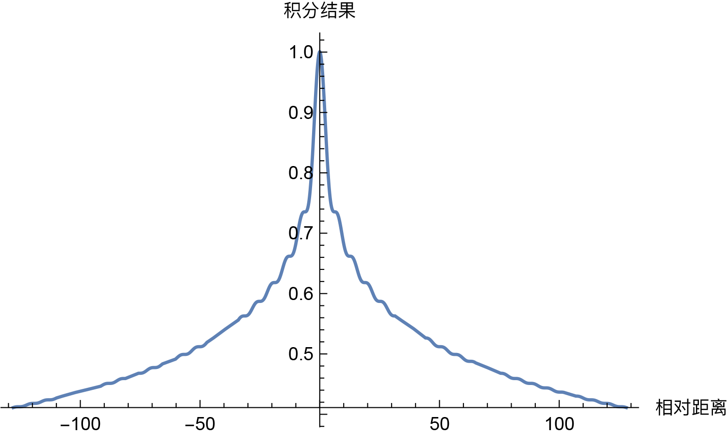
So, the question arises: must it be \theta_t = 10000^{-t} to exhibit a long-range decay trend? Of course not. In fact, for our scenario, “almost” every monotonic smooth function \theta_t on [0,1] can make the integral \int_0^1 e^{\text{i}(m-n)\theta_t} dt have an asymptotic decay trend, such as the power function \theta_t = t^{\alpha}. So, is there anything special about \theta_t = 10000^{-t}? Let’s compare some results.


Looking at it this way, except for \theta_t=t being somewhat unusual (intersecting with the horizontal axis), the others do not have any obvious differentiation. It is hard to determine which is better or worse; it’s just that power functions drop faster at short distances, while exponential functions drop faster at long distances. If \theta_t is overall closer to 0, then the overall drop is slower, and so on. It seems that \theta_t = 10000^{-t} is just a compromise choice with no particular uniqueness. If I were to choose, I would probably choose \theta_t = 1000^{-t}. Another option is to directly use \theta_i = 10000^{-2i/d} as the initial value for each \theta_i and then set it as trainable, letting the model automatically complete the fine-tuning, so there’s no need to agonize over which one to choose.
General Case
In the previous two sections, we demonstrated the idea of expressing relative position information through absolute position encoding. Combined with the constraint of long-range decay, we can “reverse-engineer” the Sinusoidal position encoding and provide other choices for \theta_i. But don’t forget, so far, our derivations have been based on the simple case of \boldsymbol{\mathcal{H}}=\boldsymbol{I}. For a general \boldsymbol{\mathcal{H}}, can the Sinusoidal position encoding still possess the above good properties?
If \boldsymbol{\mathcal{H}} is a diagonal matrix, then the above properties can be preserved to some extent. In this case: \boldsymbol{p}_m^{\top} \boldsymbol{\mathcal{H}} \boldsymbol{p}_n = \sum_{i=1}^{d/2} \boldsymbol{\mathcal{H}}_{2i,2i} \cos m\theta_i \cos n\theta_i + \boldsymbol{\mathcal{H}}_{2i+1,2i+1} \sin m\theta_i \sin n\theta_i Using the product-to-sum formulas, we get: \sum_{i=1}^{d/2} \frac{1}{2}\left(\boldsymbol{\mathcal{H}}_{2i,2i} + \boldsymbol{\mathcal{H}}_{2i+1,2i+1}\right) \cos (m-n)\theta_i + \frac{1}{2}\left(\boldsymbol{\mathcal{H}}_{2i,2i} - \boldsymbol{\mathcal{H}}_{2i+1,2i+1}\right) \cos (m+n)\theta_i We can see that it indeed contains the relative position m-n, although it might include an extra m+n term. If it’s not needed, the model can eliminate it by letting \boldsymbol{\mathcal{H}}_{2i,2i} = \boldsymbol{\mathcal{H}}_{2i+1,2i+1}. In this special case, we point out that Sinusoidal position encoding gives the model the possibility to learn relative positions; as for what specific position information is needed, that is determined by the model’s training.
In particular, for the above formula, the long-range decay property still exists. For example, the first summation, by analogy with the approximation in the previous section, is equivalent to the integral: \sum_{i=1}^{d/2} \frac{1}{2}\left(\boldsymbol{\mathcal{H}}_{2i,2i} + \boldsymbol{\mathcal{H}}_{2i+1,2i+1}\right) \cos (m-n)\theta_i \sim \int_0^1 h_t e^{\text{i}(m-n)\theta_t} dt Similarly, some estimation results for oscillatory integrals (refer to “Oscillatory integrals”, “Study Notes 3 - One-dimensional Oscillatory Integrals and Applications”, etc.) tell us that under easily achievable conditions, the integral value tends to zero as |m-n| \to \infty. Therefore, the long-range decay property can be preserved.
If \boldsymbol{\mathcal{H}} is not a diagonal matrix, then unfortunately, the above properties are difficult to reproduce. We can only hope that the diagonal part of \boldsymbol{\mathcal{H}} is the dominant term, so that the above properties can be approximately preserved. The diagonal part being dominant means that the correlation between any two dimensions of the d-dimensional vectors is relatively small, satisfying a certain degree of decoupling. For the Embedding layer, this assumption is somewhat reasonable. I checked the covariance matrices of the word Embedding matrix and the position Embedding matrix trained by BERT and found that the diagonal elements are significantly larger than the non-diagonal elements, proving that the assumption of diagonal dominance has some degree of rationality.
Discussion
Some readers might argue: even if you describe Sinusoidal position encoding as incomparable, it doesn’t change the fact that directly trained position encodings perform better than Sinusoidal position encoding. Indeed, experiments have shown that in Transformer models that have undergone sufficient pre-training like BERT, directly trained position encodings are slightly better than Sinusoidal position encoding. This is not denied. What this article aims to do is to derive why Sinusoidal position encoding can serve as an effective position from some principles and assumptions, but it doesn’t say it must be the best position encoding.
The derivation is based on some assumptions. If the derived result is not good enough, it means the assumptions do not match the actual situation well enough. So, for Sinusoidal position encoding, where might the problem lie? We can reflect on it step by step.
Step one: Taylor expansion. This depends on \boldsymbol{p} being a small quantity. I also tested this in BERT and found that the average magnitude of word Embeddings is larger than the average magnitude of position Embeddings. This suggests that the assumption that \boldsymbol{p} is a small quantity is reasonable to some extent, but how reasonable is hard to say, because although the Embedding magnitude is larger, it is not overwhelmingly so. Step two: assuming \boldsymbol{\mathcal{H}} is the identity matrix. Since we analyzed in the previous section that it is likely diagonally dominant, assuming the identity matrix might not be too big of a problem. Step three: assuming relative position is expressed through the inner product of two absolute position vectors. Intuition tells us this should be reasonable; the interaction of absolute positions should have the ability to express a certain degree of relative position information. Final step: determining \theta_i through the property of automatic long-range decay. This itself should be good, but this step has the most variables because there are too many optional forms for \theta_i, and even trainable \theta_i. It’s hard to pick the most reasonable one. Therefore, if we say Sinusoidal position encoding is not good enough, this step is very much worth reflecting on.
Summary
In summary, this article attempts to reverse-engineer Sinusoidal position encoding based on some assumptions. These assumptions have their own rationality and also some problems, so the corresponding Sinusoidal position encoding has its merits but is not flawless. Regardless, in current deep learning, being able to obtain an explicit solution for a specific problem rather than directly using brute-force fitting makes Sinusoidal position encoding a rare and noteworthy case worthy of our reflection.
Original Address: https://kexue.fm/archives/8231
For more details on reprinting, please refer to: “Scientific Space FAQ”