Nyströmformer: A Linearized Attention Scheme Based on Matrix Decomposition

Standard Attention

Standard Scaled-Dot Attention in matrix form is written as (sometimes the exponent includes a scaling factor, which we will not write explicitly here): Attention(\boldsymbol{Q},\boldsymbol{K},\boldsymbol{V}) = softmax\left(\boldsymbol{Q}\boldsymbol{K}^{\top}\right)\boldsymbol{V} Here \boldsymbol{Q}, \boldsymbol{K}, \boldsymbol{V}\in\mathbb{R}^{n\times d} (corresponding to Self Attention). Furthermore, all softmax operations in this article are normalized over the second dimension of the matrix.

In the above equation, the step \boldsymbol{Q}\boldsymbol{K}^{\top} must be calculated first before the softmax can be applied, which prevents us from using the associative law of matrix multiplication. Since \boldsymbol{Q}\boldsymbol{K}^{\top} involves the inner product of n^2 vectors, both time and space complexity are \mathcal{O}(n^2).

Linear Attention

A naive approach to linear Attention is: \left(\phi(\boldsymbol{Q})\varphi(\boldsymbol{K})^{\top}\right)\boldsymbol{V}=\phi(\boldsymbol{Q})\left(\varphi(\boldsymbol{K})^{\top}\boldsymbol{V}\right) where \phi, \varphi are activation functions with non-negative ranges. For ease of comparison, the normalization factor is not explicitly written above, highlighting only the main computational part. The complexity of the left side is still \mathcal{O}(n^2). However, since matrix multiplication is associative, we can calculate the product of the last two matrices first, reducing the overall complexity to \mathcal{O}(n).

The above equation directly defines Attention as the product of two matrices to exploit associativity. One can also (approximately) transform standard Attention into a product of matrices, as in the Performer mentioned in the next section. Furthermore, the number of matrices being multiplied is not necessarily two; for instance, Nyströmformer, introduced here, represents attention as the product of three matrices.

Performer

For Performer, it uses random projections to find matrices \tilde{\boldsymbol{Q}},\tilde{\boldsymbol{K}}\in\mathbb{R}^{n\times m} such that e^{\boldsymbol{Q}\boldsymbol{K}^{\top}}\approx \tilde{\boldsymbol{Q}}\tilde{\boldsymbol{K}}^{\top} in the softmax. Thus, standard Attention can be approximated as the linear Attention mentioned in the previous section. Details can be found in the previous blog post "Performer: Linearizing Attention Complexity with Random Projections".

Readers familiar with SVMs and kernel methods might recognize this as the core idea of kernel functions: the kernel function of two vectors in a low-dimensional space can be mapped to the inner product of two vectors in a high-dimensional space. It can also be linked to LSH (Locality Sensitive Hashing).

Dual Softmax

In the article "Exploration of Linear Attention: Does Attention Necessarily Need a Softmax?", we mentioned an interesting linear Attention that uses dual softmax to construct the Attention matrix: \left(softmax(\boldsymbol{Q}) softmax\left(\boldsymbol{K}^{\top}\right)\right)\boldsymbol{V}=softmax(\boldsymbol{Q})\left(softmax\left(\boldsymbol{K}^{\top}\right)\boldsymbol{V}\right) \label{eq:2sm} It can be proven that the Attention matrix constructed this way automatically satisfies normalization requirements. This is a simple and elegant linear Attention scheme.

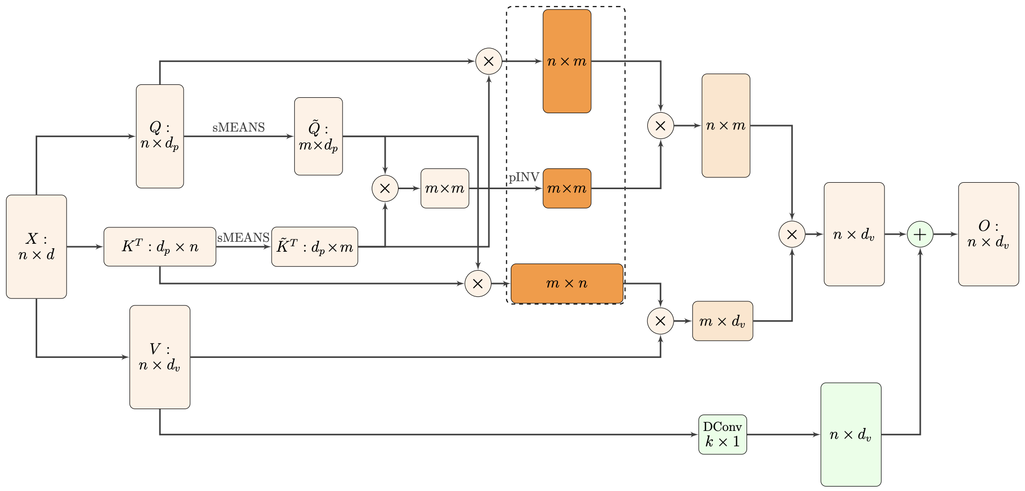
However, applying softmax directly to \boldsymbol{Q} and \boldsymbol{K}^{\top} seems a bit strange; it feels like applying softmax without a similarity (inner product) comparison might be problematic. To solve this, Nyströmformer first treats \boldsymbol{Q} and \boldsymbol{K} as n vectors of d dimensions and clusters them into m classes to obtain m cluster centers, forming matrices \tilde{\boldsymbol{Q}},\tilde{\boldsymbol{K}}\in\mathbb{R}^{m\times d}. We can then define Attention via the following formula: \left(softmax\left(\boldsymbol{Q}\tilde{\boldsymbol{K}} ^{\top}\right)softmax\left(\tilde{\boldsymbol{Q}}\boldsymbol{K}^{\top}\right)\right)\boldsymbol{V} = softmax\left(\boldsymbol{Q} \tilde{\boldsymbol{K}}^{\top}\right)\left(softmax\left(\tilde{\boldsymbol{Q}}\boldsymbol{K}^{\top}\right)\boldsymbol{V}\right) \label{eq:2sm2} The specific clustering process will be discussed later. Now, the object of the softmax is the result of an inner product, which has a clear physical meaning. Therefore, the above equation can be considered more reasonable than Equation [eq:2sm]. If we choose a relatively small m, the complexity of the right side depends linearly on n, making it a linear Attention.

Approaching the Standard

From the perspective of improving Equation [eq:2sm], Equation [eq:2sm2] has already achieved its goal. However, Nyströmformer is not limited to this; it also hopes the improved result is closer to standard Attention. To this end, observe that the attention matrix in Equation [eq:2sm2], softmax\left(\boldsymbol{Q}\tilde{\boldsymbol{K}}^{\top}\right)softmax\left(\tilde{\boldsymbol{Q}}\boldsymbol{K}^{\top}\right), is an n\times m matrix multiplied by an m\times n matrix. To fine-tune the result without increasing complexity too much, we can consider inserting an m\times m matrix \boldsymbol{M} in the middle: softmax\left(\boldsymbol{Q}\tilde{\boldsymbol{K}} ^{\top}\right) \,\boldsymbol{M}\, softmax\left(\tilde{\boldsymbol{Q}}\boldsymbol{K}^{\top}\right) How should we choose \boldsymbol{M}? A reasonable requirement is that when m=n, it should be exactly equivalent to standard Attention. In this case, \tilde{\boldsymbol{Q}}=\boldsymbol{Q}, \tilde{\boldsymbol{K}}=\boldsymbol{K}, which implies: \boldsymbol{M} = \left(softmax\left(\boldsymbol{Q}\boldsymbol{K}^{\top}\right)\right)^{-1} = \left(softmax\left(\tilde{\boldsymbol{Q}}\tilde{\boldsymbol{K}}^{\top}\right)\right)^{-1} For a general m, \left(softmax\left(\tilde{\boldsymbol{Q}}\tilde{\boldsymbol{K}}^{\top}\right)\right)^{-1} is precisely an m\times m matrix. Thus, choosing it as \boldsymbol{M} is at least reasonable in terms of matrix operations. Based on the special case where m=n, we "boldly" speculate that choosing it as \boldsymbol{M} makes the new Attention mechanism closer to standard Attention. Therefore, Nyströmformer ultimately chooses: softmax\left(\boldsymbol{Q}\tilde{\boldsymbol{K}} ^{\top}\right) \, \left(softmax\left(\tilde{\boldsymbol{Q}}\tilde{\boldsymbol{K}}^{\top}\right)\right)^{-1} \, softmax\left(\tilde{\boldsymbol{Q}}\boldsymbol{K}^{\top}\right) as the Attention matrix. Since it is the product of three small matrices, it can be transformed into linear Attention via the associative law.

However, there is a theoretical detail to supplement: the above formula involves matrix inversion, and softmax\left(\tilde{\boldsymbol{Q}}\tilde{\boldsymbol{K}}^{\top}\right) might not be invertible. Of course, in practice, the probability of a real square matrix being non-invertible is almost zero (non-invertibility means the determinant is exactly 0; from a probability standpoint, being non-zero is much more likely). Thus, this case can be ignored in experiments, but it must be addressed theoretically. This is simple: if a matrix is non-invertible, replace the inverse with the "pseudo-inverse" (denoted by ^{\dagger}), which exists for any matrix and equals the inverse when the matrix is invertible.

Therefore, the final Attention matrix form for Nyströmformer is: softmax\left(\boldsymbol{Q}\tilde{\boldsymbol{K}} ^{\top}\right) \, \left(softmax\left(\tilde{\boldsymbol{Q}}\tilde{\boldsymbol{K}}^{\top}\right)\right)^{\dagger} \, softmax\left(\tilde{\boldsymbol{Q}}\boldsymbol{K}^{\top}\right) \label{eq:2sm3}

Iterative Matrix Inversion

Theoretically, Equation [eq:2sm3] has reached the goal, but implementation requires handling practical details, such as how to compute the pseudo-inverse. The pseudo-inverse is also called the generalized inverse or Moore-Penrose inverse. The standard way to compute it is via SVD. Let the SVD of matrix \boldsymbol{A} be \boldsymbol{U} \boldsymbol{\Lambda} \boldsymbol{V}^{\top}; then its pseudo-inverse is: \boldsymbol{A}^{\dagger} = \boldsymbol{V} \boldsymbol{\Lambda}^{\dagger} \boldsymbol{U}^{\top} where the pseudo-inverse of the diagonal matrix \boldsymbol{\Lambda}, \boldsymbol{\Lambda}^{\dagger}, is obtained by taking the reciprocal of all non-zero diagonal elements. While SVD is theoretically simple, its computational cost is high, and it is not easy to compute gradients, making it an imperfect way to implement the pseudo-inverse.

Nyströmformer adopts an iterative approximation method for the inverse. Specifically, it uses the iterative algorithm provided in the paper "Chebyshev-type methods and preconditioning techniques":

If the initial matrix \boldsymbol{V}_0 satisfies \Vert \boldsymbol{I} - \boldsymbol{A} \boldsymbol{V}_0\Vert < 1, then for the following iterative format: \begin{aligned} \boldsymbol{V}_{n+1} =&\,\left[\boldsymbol{I} + \frac{1}{4}\left(\boldsymbol{I} - \boldsymbol{V}_n \boldsymbol{A}\right)\left(3 \boldsymbol{I} - \boldsymbol{V}_n \boldsymbol{A}\right)^2\right] \boldsymbol{V}_n \\ =&\,\frac{1}{4} \boldsymbol{V}_n (13 \boldsymbol{I} - \boldsymbol{A} \boldsymbol{V}_n (15 \boldsymbol{I} - \boldsymbol{A} \boldsymbol{V}_n (7 \boldsymbol{I} - \boldsymbol{A} \boldsymbol{V}_n))) \end{aligned} it holds that \lim\limits_{n\to\infty} \boldsymbol{V}_n = \boldsymbol{A}^{\dagger}.

Here \Vert\cdot\Vert can be any matrix norm. A simple initial value satisfying the condition can be: \boldsymbol{V}_0 = \frac{\boldsymbol{A}^{\top}}{\Vert\boldsymbol{A}\Vert_1 \Vert\boldsymbol{A}\Vert_{\infty}} = \frac{\boldsymbol{A}^{\top}}{\left(\max\limits_j\sum\limits_i |A_{i,j}|\right)\left(\max\limits_i\sum\limits_j |A_{i,j}|\right)} In the Nyströmformer paper, the authors use this initial value and iterative format, taking the result after 6 iterations to replace \boldsymbol{A}^{\dagger}. Six iterations might seem like a lot, but since the chosen m is small (64 in the paper) and the process only involves matrix multiplication, the computational cost is not too high, and gradients are easy to compute. This solves the pseudo-inverse problem. The paper refers to this iterative process as pINV.

Pooling as Clustering

Another problem to solve is the choice of clustering method. A direct idea is to use K-Means. However, similar to the pseudo-inverse problem, designing a model requires considering both forward computation and backpropagation for gradients. K-Means involves an \mathop{\text{argmin}} operation, which cannot yield meaningful gradients. It would need to be "softened" to be embedded in the model, which essentially becomes the "dynamic routing" process of Capsule Networks, discussed in "Another New Year Feast: From K-Means to Capsule". The main issue is that K-Means is an iterative process, requiring several iterations to ensure effectiveness, which significantly increases computation.

Nyströmformer chooses a very simple solution: assuming the sequence length n is a multiple of m (if not, pad with zero vectors), it takes the average of every n/m vectors of \boldsymbol{Q} and \boldsymbol{K} as the vectors of \tilde{\boldsymbol{Q}} and \tilde{\boldsymbol{K}}. This operation is called Adaptive Average Pooling (referred to as Segment-Means or sMEANS in the original paper). It is a pooling method that uses an adaptive window size to ensure the pooled feature matrix has a fixed shape. Nyströmformer’s experiments show that complex clustering is unnecessary; simple adaptive pooling achieves very competitive results. Moreover, choosing m=64 (roughly the same as the original d) is much better than Performer, which requires m to be several times larger than d.

However, a clear disadvantage of adaptive pooling is that it "mixes" information within each interval, which prevents it from avoiding future information leakage, thus making it unsuitable for autoregressive generation (like language models or Seq2Seq decoders). This is a common drawback of any model using pooling techniques.

Performance and Effectiveness

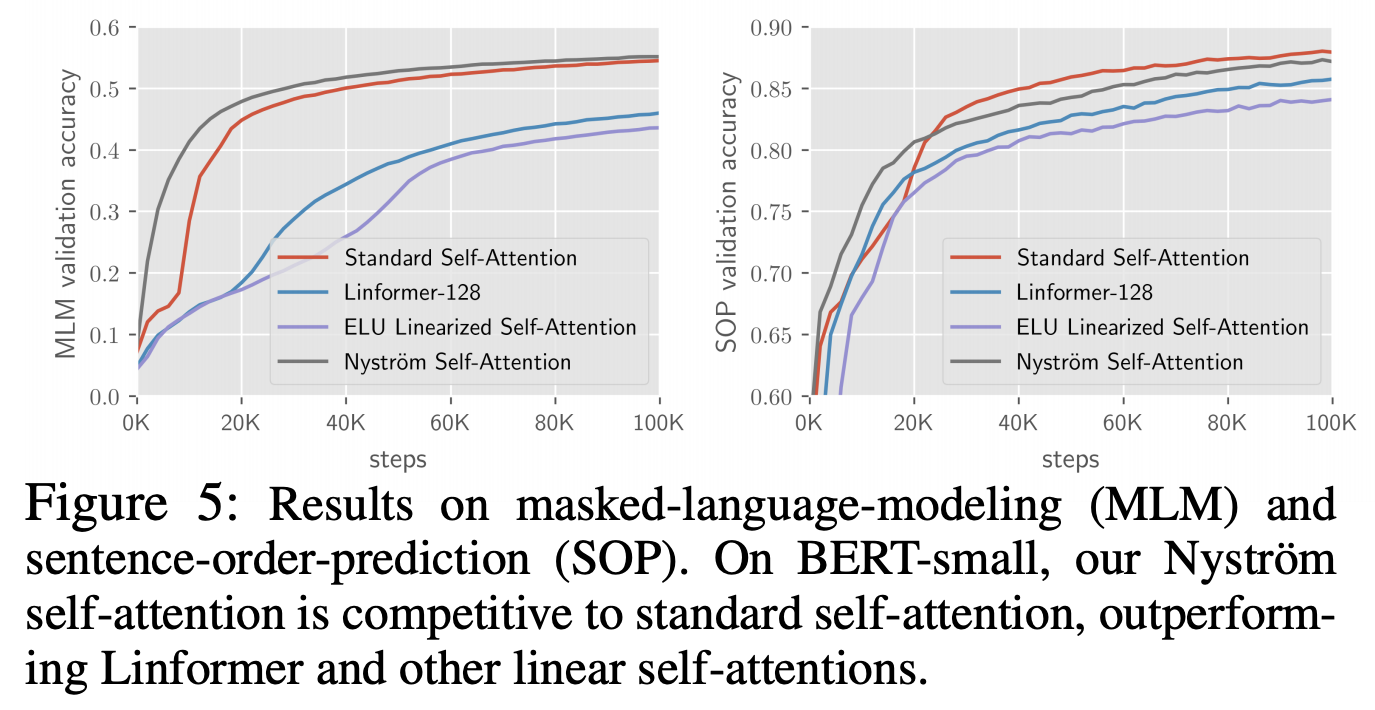
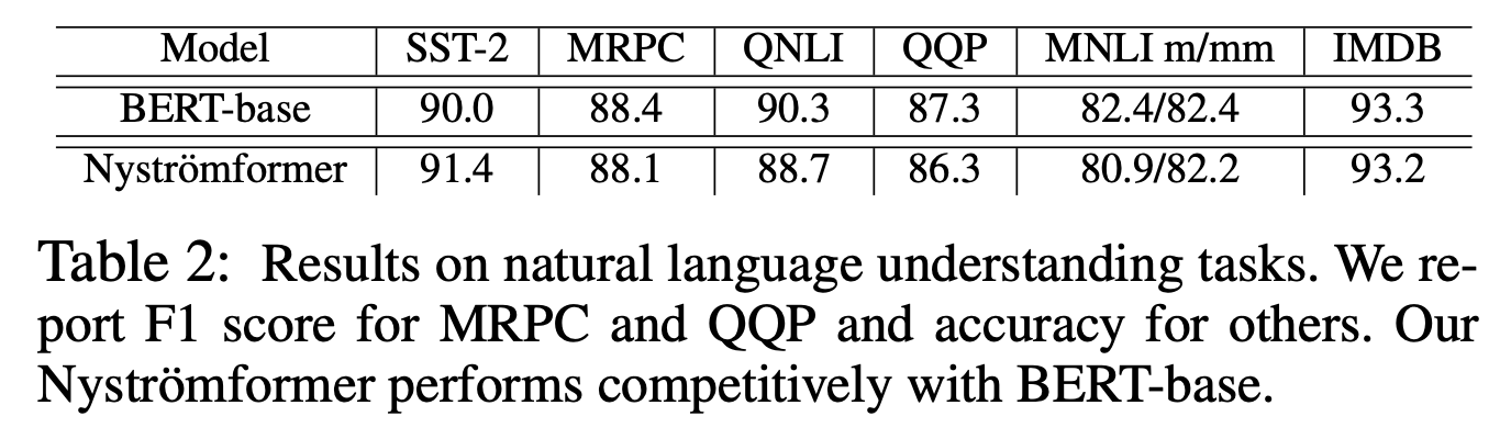
Likely limited by computing power, the original paper’s experiments are not extremely extensive. They mainly replaced standard Attention in small and base versions of BERT with Nyströmformer for comparison. The results are shown in the two figures below. One is the pre-training effect, where it is interesting to note that Nyströmformer performs even better than standard Attention on the MLM task. The other shows fine-tuning results on downstream tasks, indicating competitiveness with standard Attention (i.e., BERT).

However, the original paper did not compare Nyströmformer with similar models, providing only the complexity comparison chart below, which makes it harder to highlight Nyströmformer’s specific competitive edge:

Personal Thoughts

Overall, Nyströmformer’s approach to approximating standard Attention via linearization is quite novel and worth studying. However, the pseudo-inverse part feels a bit unnatural; this might be a point for future improvement—if it could be done without approximation, it would be perfect. Additionally, how to quantitatively estimate the error between Nyströmformer and standard Attention is a theoretical question worth considering.

From the experiments, Nyströmformer appears competitive, especially with MLM results surpassing standard Attention, showing its potential. As mentioned, the inclusion of Pooling means it cannot perform autoregressive generation, which is a significant drawback. I haven’t thought of a good way to remedy this yet.

Compared to Performer, Nyströmformer removes the randomness in the linearization process. Since Performer achieves linearization through random projections, it inevitably introduces randomness. For some "perfectionist" readers, this randomness might be hard to accept, whereas Nyströmformer does not have this issue, which is a highlight.

The Nyström Method

Some readers might want to learn about the Nyström method itself. To understand it, one first needs a basic understanding of the CUR decomposition of a matrix.

Most people have heard of SVD decomposition, \boldsymbol{A}=\boldsymbol{U} \boldsymbol{\Lambda} \boldsymbol{V}^{\top}, where \boldsymbol{U}, \boldsymbol{V} are orthogonal and \boldsymbol{\Lambda} is diagonal. Note that orthogonal matrices are dense, so when \boldsymbol{A} is very large, the cost of computing and storing SVD is high (even with approximations). If \boldsymbol{A} is large but sparse, its SVD might be much more expensive than the original matrix. Thus, CUR decomposition was born. it aims to select k columns to form matrix \boldsymbol{C}, k rows to form matrix \boldsymbol{R}, and insert a k\times k matrix \boldsymbol{U} such that: \boldsymbol{A} \approx \boldsymbol{C}\boldsymbol{U}\boldsymbol{R} Since \boldsymbol{C} and \boldsymbol{R} are parts of the original matrix, they inherit its sparsity. For more on CUR decomposition, readers can refer to the "Dimensionality Reduction" section of Stanford’s CS246 course. Unlike SVD, CUR decomposition is more of a decomposition philosophy than a specific algorithm. It has different implementations, and the Nyström method is one of them, with the form: \begin{pmatrix}\boldsymbol{A} & \boldsymbol{B} \\ \boldsymbol{C} & \boldsymbol{D}\end{pmatrix} \approx \begin{pmatrix}\boldsymbol{A} & \boldsymbol{B} \\ \boldsymbol{C} & \boldsymbol{C}\boldsymbol{A}^{\dagger}\boldsymbol{B}\end{pmatrix} = \begin{pmatrix}\boldsymbol{A} \\ \boldsymbol{C}\end{pmatrix} \boldsymbol{A}^{\dagger} \begin{pmatrix}\boldsymbol{A} & \boldsymbol{B}\end{pmatrix} where \begin{pmatrix}\boldsymbol{A} \\ \boldsymbol{C}\end{pmatrix} and \begin{pmatrix}\boldsymbol{A} & \boldsymbol{B}\end{pmatrix} are the selected column and row matrices. For convenience, we assume the selected rows and columns are arranged at the front. Nyströmformer does not directly use the Nyström method (in fact, it cannot be applied directly, as described in the original paper), but rather borrows the decomposition philosophy of the Nyström method.

Regarding the Nyström method, the original paper primarily cites "Improving CUR Matrix Decomposition and the Nyström Approximation via Adaptive Sampling", but I do not recommend this for beginners. Instead, I recommend "Matrix Compression using the Nyström Method" and "Using the Nyström Method to Speed Up Kernel Machines".

It should be noted that I am also new to CUR decomposition and the Nyström method, so there may be misunderstandings. Readers should discern for themselves, and I welcome corrections from those familiar with the theory.