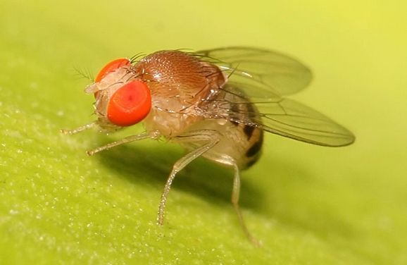
Some readers may have recently noticed the ICLR 2021 paper "Can a Fruit Fly Learn Word Embeddings?". The paper describes a binarized word vector model built on bionic principles (specifically, the olfactory circuit of the fruit fly). Actually, the algorithmic part of the paper is not particularly difficult to read. The main confusion for most readers after finishing the paper might be: "What does this have to do with fruit flies?" or "Was the author really inspired by fruit flies?" In this article, let us trace the origins of this algorithm and attempt to answer how this word vector model got connected to fruit flies.
BioWord
The original paper did not give this word vector model a specific name. For convenience, I will take the liberty of calling it "BioWord." Generally speaking, the content of the paper consists of three main parts:
1. Constructing a bag-of-words representation vector for each n-gram;
2. Executing the BioHash algorithm on these n-gram vectors to obtain so-called (binarized) static/dynamic word vectors;
3. "Striving hard" to tell a story.
We will introduce BioHash later; in short, it is an existing vector binarization algorithm. From these three points, it can be seen that the word vector model itself does not have an obvious connection to bionics or fruit flies. Even if there is a connection, it should reside within the BioHash algorithm. However, since this paper is not the one that proposed the BioHash algorithm, talking too much about bionics feels a bit forced. Let’s explain these points in more detail.
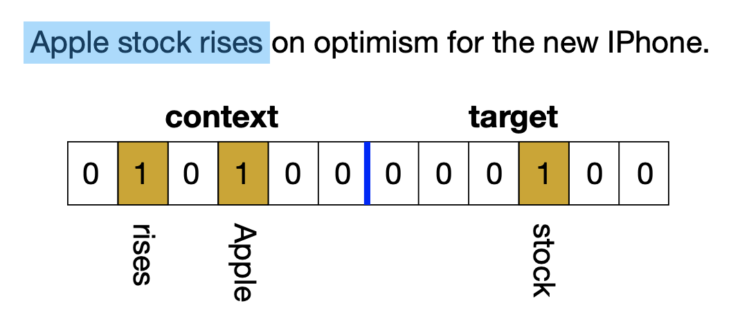
First, constructing a bag-of-words representation for each n-gram is a very simple approach. The result is a 2V-dimensional binary vector (i.e., a 0/1 vector), where V is the vocabulary size. As shown in the figure below, the first V dimensions represent the context part, where 1 indicates the word appeared in the context; the latter V dimensions are a one-hot vector representing the center word. Then, the authors made a slight adjustment to the BioHash algorithm (though they did not clearly explain why they made this modification, and I cannot see how to interpret it). After BioHash, each n-gram vector is mapped to a K-dimensional 0/1 vector, where each vector has a (fixed number of) k ones.
Finally, why do I say the authors "strived hard" to tell a story? First, as mentioned, talking too much about bionics seems forced. Second, the authors compared BioWord with word vector models like Word2Vec and GloVe, and the performance was generally inferior to them. Third, as a word vector binarization algorithm, BioWord’s performance shows no advantage compared to existing methods like RandExp or LSH. If it were just that, it might be fine, but what makes it more awkward is that the authors also forcibly compared it with BERT to highlight their "advantages."
The authors first introduced the concepts of static and dynamic word vectors. If the first V dimensions of the bag-of-words vector are all 0, then the mapped K-dimensional vector is the static word vector for that word. If the first V dimensions depend on the context, then the mapped K-dimensional vector is called the dynamic word vector (similar to BERT). But this concept is hardly sophisticated. By this logic, even with Word2Vec, if you take the average word vector of the context and concatenate it with the center word vector, it becomes a dynamic word vector. This is nothing more than a talking point, and the experimental results showed no advantage. Furthermore, as a word vector model, the authors compared their training cost with BERT to highlight their advantage, which was quite embarrassing. This also shows how much "painstaking effort" the authors put into telling this story.
BioHash
BioHash comes from the paper "Bio-Inspired Hashing for Unsupervised Similarity Search". It is a method for vector binarization. Unlike traditional LSH, it is data-dependent and "tailor-made" for specific datasets, so it usually yields better and sparser binary vectors.
Given a set of vectors \{\boldsymbol{x}_i\}_{i=1}^N, the BioHash algorithm is roughly as follows:
1. Use K-Means to cluster \{\boldsymbol{x}_i\}_{i=1}^N into K clusters, obtaining K vector centers;
2. Map each \boldsymbol{x}_i to a K-dimensional 0/1 vector, where the positions corresponding to the k clusters closest to \boldsymbol{x}_i are set to 1, and the rest are 0.
The reason I say "roughly" is that there are some discrepancies in the algorithmic details. First, the distance used in the clustering process is not Euclidean distance but a normalized inner product, i.e., d(\boldsymbol{x}, \boldsymbol{w}) = -\langle \boldsymbol{x}, \boldsymbol{w} / \Vert\boldsymbol{w}\Vert\rangle. We used this approach before when exploring Capsules; readers can refer to "Another New Year’s Eve Feast: From K-Means to Capsule". Second, when solving for cluster centers, SGD is used instead of the conventional EM algorithm. I don’t quite understand this point; although SGD can be done in small batches and is more memory-friendly, theoretically, the EM algorithm can also be executed in batches without exploding memory. Finally, a point I completely fail to understand is that the authors use the normalized inner product -\langle \boldsymbol{x}, \boldsymbol{w} / \Vert\boldsymbol{w}\Vert\rangle as the distance during clustering, but when determining the assignment of each sample, they use the unnormalized inner product -\langle \boldsymbol{x}, \boldsymbol{w}\rangle as the distance, which is truly baffling.
Of course, putting aside the details of BioHash, its performance is quite impressive. So, if there is a suitable scenario, BioHash is worth learning from. Attentive readers may notice that several authors of BioWord and BioHash are the same. In fact, they all come from the same laboratory. Thus, it is not hard to understand BioWord’s intention to inherit from BioHash. However, applying BioHash to word vector construction is, in my opinion, neither motivated well nor particularly beautiful in terms of reported results.
FlyHash
After talking for so long, we still haven’t addressed the question in the title: What is the connection between BioWord and fruit flies? Or where does BioHash reflect similarity to fruit flies? Tracing the references of BioHash reveals that BioHash is actually an improvement on an algorithm called FlyHash. Therefore, to find the source, we must look at FlyHash.
As the name suggests, FlyHash is a new vector binarization method inspired by the olfactory circuit of the fruit fly. it is more efficient than conventional LSH. For readers unfamiliar with LSH, we will introduce it later; here, let’s introduce FlyHash directly. In fact, both FlyHash and LSH follow the idea of "random projection + binarization," but the fruit fly inspired a new optimization direction: high dimensionality + low activation.
Specifically, let the original data be \boldsymbol{x}_i \in \mathbb{R}^{D}. FlyHash chooses a random binary matrix \boldsymbol{W}\in\{0,1\}^{D\times K} (fixed once chosen), where generally K > D (high dimensionality). After projection, \boldsymbol{x}_i \boldsymbol{W} is a K-dimensional vector. Then, a WTA (Winner Take All) operation is performed to achieve "low activation"—"set the k largest elements of \boldsymbol{x}_i \boldsymbol{W} to 1 and the rest to 0." This results in a binary vector with k ones and K-k zeros, which serves as the Hash vector for \boldsymbol{x}_i.
Since there are only a limited number of k activation values, even if the dimensionality is increased, the storage and retrieval costs do not increase; instead, the performance improves. This is the benefit of the "high dimensionality + low activation" idea brought by the fruit fly. FlyHash was first published in the Science paper "A neural algorithm for a fundamental computing problem". For details on the fruit fly olfactory circuit’s "high dimensionality + low activation," please refer to that paper. Later, the paper "Improving Similarity Search with High-dimensional Locality-sensitive Hashing" further refined the theoretical part. These two papers are part of the same lineage.
So, now we can answer "how it got connected to fruit flies." Essentially, any algorithm that includes the "high dimensionality + low activation" idea in the binarization process can be said to be "Inspired by Fly." Since FlyHash uses random projection to get the final result, it must be projected to a sufficiently high dimension to ensure performance. BioHash, being trained on specific datasets, often does not require as many dimensions as FlyHash and performs better. However, BioHash also clearly embodies the "Winner Take All" idea, so it is also called "Inspired by Fly." Since BioWord uses BioHash, it also claims to be "Inspired by Fly."
LSH
Finally, let’s briefly introduce LSH (Locality Sensitive Hashing) for readers who are not familiar with it. A complete explanation of LSH could be very long; here, I will mainly mention the parts closely related to FlyHash.
Simply put, LSH is an algorithm that binarizes vectors such that the binarized vectors approximately preserve the metric. A common scheme is to use random projection to (approximately) preserve the invariance of the cosine value. From previous articles "Distribution of the Angle Between Two Random Vectors in n-Dimensional Space" and "Understanding Model Parameter Initialization Strategies from a Geometric Perspective", we know that any two Gaussian random vectors in high-dimensional space are almost orthogonal. If we sample DK random numbers from \mathcal{N}(0,1/n) to form a matrix \boldsymbol{W}\in\mathbb{R}^{D\times K}, it is "almost" an orthogonal matrix. Consequently, when two original vectors \boldsymbol{x}_i, \boldsymbol{x}_j\in\mathbb{R}^{D} are multiplied by \boldsymbol{W}, they become two K-dimensional vectors, and their angle remains approximately unchanged: \cos(\boldsymbol{x}_i \boldsymbol{W}, \boldsymbol{x}_j \boldsymbol{W})\approx \cos(\boldsymbol{x}_i, \boldsymbol{x}_j) Thus, if the retrieval metric is the cosine value, we can use the projected \boldsymbol{x} \boldsymbol{W} instead of the original vector \boldsymbol{x} for approximate retrieval. Furthermore, binarizing the result basically preserves the cosine value: \boldsymbol{x}\quad\to\quad\text{sgn}(\boldsymbol{x} \boldsymbol{W}) where \text{sgn} is the sign function, changing values greater than 0 to 1 and values less than or equal to 0 to -1. This maps the original vector to a binary vector. Here, the target dimension K is generally not larger than D, and due to the randomness of the projection, we can roughly assume that 1s and -1s each make up half of the result. This is clearly different from FlyHash’s "high dimensionality + low activation," because whether you treat 1 or -1 as the activation value, the count is roughly the same, which cannot be called "low activation."
Although the above introduction is just a heuristic guide, it is actually supported by rigorous probability theory (related theoretical analysis was also done in "Performer: Linearizing Attention Complexity with Random Projections"). Therefore, LSH is a rigorous and quantifiable set of algorithms, not just a random approximation. After binarizing vectors, we can treat them as a bag-of-words model (even if the original ones were continuous vectors) and build indices to speed up retrieval, such as inverted indices. This is the significance of vector binarization. Vector retrieval libraries like Faiss include LSH algorithms.
Summary
This article traced the origins of a binarized word vector model and explored how it actually connects to fruit flies. From this, we can also understand the ideas and connections behind vector binarization methods such as BioHash, FlyHash, and LSH. This article is also a first attempt at a reverse-chronological writing style; I hope readers enjoy it.
Please include the original address when reposting: https://kexue.fm/archives/8159
For more detailed reposting matters, please refer to: "Scientific Space FAQ"