Although Transformer-based models have conquered most fields of NLP, RNN models such as LSTM and GRU still have their unique value in certain scenarios. Therefore, RNNs remain a model worth studying thoroughly. The analysis of RNN gradients is an excellent example of thinking about and analyzing models from an optimization perspective, and it is worth careful consideration. As you may know, questions like "Why can LSTM solve the gradient vanishing/exploding problem?" are still popular interview questions today...
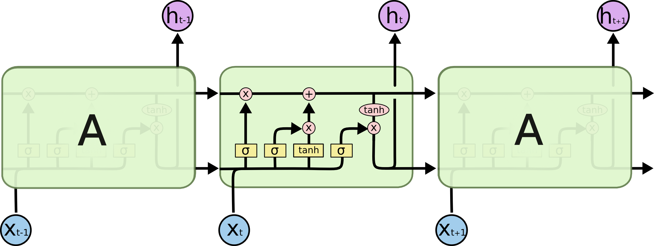
Many netizens have provided answers to such questions. However, after searching through various articles (including some answers on Zhihu, columns, and classic English blogs), I found that there are no particularly good answers: some derivation notations are chaotic, some arguments do not highlight the key points, and overall they feel insufficiently clear and self-consistent. To this end, I will attempt to provide my own understanding for your reference.
RNN and its Gradient
The unified definition of an RNN is: h_t = f\left(x_t, h_{t-1};\theta\right) where h_t is the output at each step, which is jointly determined by the current input x_t and the previous output h_{t-1}, and \theta represents the trainable parameters. In the most basic analysis, we can assume that h_t, x_t, \theta are all one-dimensional. This allows us to gain the most intuitive understanding, and the results still have reference value for high-dimensional cases. We consider the gradient because our current mainstream optimizers are still gradient descent and its variants, which require the models we define to have reasonable gradients. We can obtain: \frac{d h_t}{d\theta} = \frac{\partial h_t}{\partial h_{t-1}}\frac{d h_{t-1}}{d\theta} + \frac{\partial h_t}{\partial \theta} As we can see, the gradient of an RNN is actually also an RNN; the current gradient \frac{d h_t}{d\theta} is a function of the previous gradient \frac{d h_{t-1}}{d\theta} and the current operation’s gradient \frac{\partial h_t}{\partial \theta}. At the same time, we can see from the above equation that the phenomenon of gradient vanishing or exploding is almost inevitable: when \left|\frac{\partial h_t}{\partial h_{t-1}}\right| < 1, it means the historical gradient information decays, so the gradient will inevitably vanish as the number of steps increases (similar to \lim_{n\to\infty} 0.9^n \to 0); when \left|\frac{\partial h_t}{\partial h_{t-1}}\right| > 1, the historical gradient information gradually strengthens, so the gradient will inevitably explode as the number of steps increases (similar to \lim_{n\to\infty} 1.1^n \to \infty). It is impossible for \left|\frac{\partial h_t}{\partial h_{t-1}}\right| to be exactly 1 all the time. Of course, it is possible that it is greater than 1 at some moments and less than 1 at others, eventually stabilizing around 1, but the probability of this is very small and requires very careful model design.
Therefore, as the number of steps increases, gradient vanishing or exploding is almost inevitable; we can only alleviate this problem for a finite number of steps.
Vanishing or Exploding?
Having said that, we haven’t clarified one question: what exactly is gradient vanishing/exploding in an RNN? Gradient explosion is easy to understand—the gradient value diverges and may even become NaN. Does gradient vanishing mean the gradient becomes zero? Not exactly. We just said that gradient vanishing occurs when \left|\frac{\partial h_t}{\partial h_{t-1}}\right| is consistently less than 1, causing historical gradients to decay continuously, but this doesn’t mean the total gradient becomes zero. Specifically, iterating further, we have: \begin{aligned}\frac{d h_t}{d\theta} &= \frac{\partial h_t}{\partial h_{t-1}}\frac{d h_{t-1}}{d\theta} + \frac{\partial h_t}{\partial \theta}\\ &= \frac{\partial h_t}{\partial \theta}+\frac{\partial h_t}{\partial h_{t-1}}\frac{\partial h_{t-1}}{\partial \theta}+\frac{\partial h_t}{\partial h_{t-1}}\frac{\partial h_{t-1}}{\partial h_{t-2}}\frac{\partial h_{t-2}}{\partial \theta}+\dots\\ \end{aligned} Clearly, as long as \frac{\partial h_t}{\partial \theta} is not zero, the probability of the total gradient being zero is very small. However, if we continue iterating, the coefficient in front of the term \frac{\partial h_1}{\partial \theta} is the product of t-1 terms \frac{\partial h_t}{\partial h_{t-1}}\frac{\partial h_{t-1}}{\partial h_{t-2}}\cdots\frac{\partial h_2}{\partial h_1}. If their absolute values are all less than 1, the result will tend toward 0. Consequently, \frac{d h_t}{d\theta} contains almost no information from the initial gradient \frac{\partial h_1}{\partial \theta}. This is the true meaning of gradient vanishing in RNNs: the further away from the current time step, the less significant the feedback gradient signal becomes, and it may eventually have no effect at all. This means that the RNN’s ability to capture long-distance semantics fails.
Simply put, if your optimization process has nothing to do with long-distance feedback, how can you guarantee that the learned model can effectively capture long distances?
Mathematical Formulas
The above text provided a general analysis. Next, we will analyze specific RNNs. Before that, we need to review several mathematical formulas that we will use multiple times in the following derivations: \begin{aligned} &\tanh x = 2\sigma(2x) - 1\\ &\sigma(x) = \frac{1}{2}\left(\tanh \frac{x}{2} + 1\right)\\ &(\tanh x)' = 1 - \tanh^2 x\\ &\sigma'(x) = \sigma(x)\left(1 - \sigma(x)\right) \end{aligned} where \sigma(x) = 1/(1+e^{-x}) is the sigmoid function. These formulas essentially state one thing: \tanh x and \sigma(x) are basically equivalent, and their derivatives can both be expressed in terms of themselves.
Simple RNN Analysis
First to appear is the primitive Simple RNN. Its formula is: h_t = \tanh \left(Wx_t + Uh_{t-1} + b\right) where W, U, b are parameters to be optimized. Seeing this, a natural question arises: why use \tanh as the activation function instead of the more popular \text{ReLU}? This is a good question, and we will answer it shortly.
From the previous discussion, we know that whether the gradient vanishes or explodes mainly depends on \left|\frac{\partial h_t}{\partial h_{t-1}}\right|, so we calculate: \frac{\partial h_t}{\partial h_{t-1}} = \left(1-h_t^2\right)U\label{eq:rnn-g} Since we cannot determine the range of U, \left|\frac{\partial h_t}{\partial h_{t-1}}\right| could be less than 1 or greater than 1, so the risk of gradient vanishing/exploding exists. Interestingly, if |U| is very large, then h_t will correspondingly be very close to 1 or -1, which in turn makes (1-h_t^2)U smaller. In fact, it can be strictly proven that if h_{t-1} \neq 0 is fixed, then (1-h_t^2)U as a function of U is bounded. This means that no matter what U is, it will not exceed a fixed constant.
Thus, we can answer why \tanh is used as the activation function: because after using \tanh, the corresponding gradient \frac{\partial h_t}{\partial h_{t-1}} is bounded. Although this bound might not be 1, the probability of a bounded quantity not exceeding 1 is generally higher than that of an unbounded quantity, thus the risk of gradient explosion is lower. In contrast, if \text{ReLU} is used, its derivative on the positive axis is always 1, making \frac{\partial h_t}{\partial h_{t-1}}=U unbounded, which increases the risk of gradient explosion.
Therefore, the main purpose of using \tanh instead of \text{ReLU} in RNNs is to alleviate the risk of gradient explosion. Of course, this alleviation is relative; there is still a possibility of explosion even with \tanh. In fact, the most fundamental method for dealing with gradient explosion is parameter clipping or gradient clipping. In other words, if I manually clip U to the range [-1, 1], can’t I guarantee that the gradient won’t explode? Some readers might then ask: since clipping can solve the problem, can we use \text{ReLU}? Indeed, with good initialization and parameter/gradient clipping schemes, \text{ReLU}-based RNNs can also be trained well. However, we still prefer \tanh because its corresponding \frac{\partial h_t}{\partial h_{t-1}} is bounded, meaning we don’t have to clip too aggressively, which might allow for better model fitting capability.
LSTM Results
Of course, while clipping works, it is ultimately a last resort. Moreover, clipping only solves the gradient explosion problem and cannot solve gradient vanishing. If we can solve this problem through model design, that would naturally be best. The legendary LSTM is such a design. Is this true? Let’s analyze it.
The update formulas for LSTM are quite complex: \begin{aligned} f_{t} & = \sigma \left( W_{f} x_{t} + U_{f} h_{t - 1} + b_{f} \right) \\ i_{t} & = \sigma \left( W_{i} x_{t} + U_{i} h_{t - 1} + b_{i} \right) \\ o_{t} & = \sigma \left( W_{o} x_{t} + U_{o} h_{t - 1} + b_{o} \right) \\ \hat{c}_t & = \tanh \left( W_{c} x_{t} + U_{c} h_{t - 1} + b_{c} \right)\\ c_{t} & = f_{t} \circ c_{t - 1} + i_{t} \circ \hat{c}_t \\ h_{t} & = o_{t} \circ \tanh \left( c_{t} \right)\end{aligned} We can calculate \frac{\partial h_t}{\partial h_{t-1}} as before, but since h_{t} = o_{t} \circ \tanh \left( c_{t} \right), analyzing c_{t} is equivalent to analyzing h_{t}, and calculating \frac{\partial c_t}{\partial c_{t-1}} is simpler.
Assuming the 1D case, we have: \frac{\partial c_t}{\partial c_{t-1}}=f_t + c_{t-1}\frac{\partial f_t}{\partial c_{t-1}}+ \hat{c}_{t}\frac{\partial i_t}{\partial c_{t-1}}+ i_{t}\frac{\partial \hat{c}_t}{\partial c_{t-1}} The first term f_t is the "forget gate". As discussed below, the other three terms are usually secondary, making f_t the "main term". Since f_t \in [0, 1], the risk of gradient explosion is small. Whether the gradient vanishes depends on whether f_t is close to 1. There is a self-consistent conclusion: if the task relies on historical information, f_t will be close to 1, and the historical gradient will not vanish; if f_t is close to 0, the task does not rely on history, so gradient vanishing is acceptable.
Now, let’s see if the other three terms are indeed secondary. Each is a product of a term and a partial derivative of a \sigma or \tanh function. For the second term, substituting h_{t-1} = o_{t-1} \tanh \left( c_{t-1} \right): c_{t-1}\frac{\partial f_t}{\partial c_{t-1}}=f_t \left(1 - f_t\right) o_{t-1} \left(1-\tanh^2 c_{t-1}\right)c_{t-1}U_f Since f_t, 1-f_t, o_{t-1} are in [0, 1] and |(1-\tanh^2 c_{t-1})c_{t-1}| < 0.45, this term is U_f multiplied by four "gates", making it very small unless initialization is poor. Compared to the simple RNN gradient [eq:rnn-g], it has three more gates.
The other two terms are similar: \begin{aligned} \hat{c}_{t}\frac{\partial i_t}{\partial c_{t-1}}=&\,i_t \left(1 - i_t\right) o_{t-1} \left(1-\tanh^2 c_{t-1}\right)\hat{c}_{t}U_i\\ i_{t}\frac{\partial \hat{c}_t}{\partial c_{t-1}}=&\,\left(1 - \hat{c}_t^2\right) o_{t-1} \left(1-\tanh^2 c_{t-1}\right)i_{t}U_c \end{aligned} These terms also contain more "gates" and are compressed further. Thus, f_t dominates. Its range [0, 1] ensures low explosion risk, and its value reflects historical dependency, naturally preserving gradients. Thus, LSTM alleviates both problems.
A Look at GRU
Finally, let’s analyze GRU. Its operations are: \begin{aligned} z_{t} & = \sigma \left( W_{z} x_{t} + U_{z} h_{t - 1} + b_{z} \right) \\ r_{t} & = \sigma \left( W_{r} x_{t} + U_{r} h_{t - 1} + b_{r} \right) \\ \hat{h}_t & = \tanh \left( W_{h} x_{t} + U_{h} (r_t \circ h_{t - 1}) + b_{c} \right)\\ h_{t} & = \left(1 - z_{t}\right) \circ h_{t - 1} + z_{t} \circ \hat{h}_t \end{aligned} An extreme version combines r_t and z_t: \begin{aligned} r_{t} & = \sigma \left( W_{r} x_{t} + U_{r} h_{t - 1} + b_{r} \right) \\ \hat{h}_t & = \tanh \left( W_{h} x_{t} + U_{h} (r_t \circ h_{t - 1}) + b_{c} \right)\\ h_{t} & = \left(1 - r_{t}\right) \circ h_{t - 1} + r_{t} \circ \hat{h}_t \end{aligned} In GRU, h_t stays in [-1, 1] because it is a weighted average of h_{t-1} and \hat{h}_t \in [-1, 1]. Calculating the derivative: \begin{aligned} \frac{\partial h_t}{\partial h_{t-1}} =& 1 - z_t - z_t (1-z_t) h_{t-1} U_z + z_t (1-z_t) \hat{h}_{t} U_z \\ & + \left(1-\hat{h}_{t}^2\right)r_t\left(1 + (1 - r_t)h_{t-1}U_r\right) z_t U_h \end{aligned} The results are similar to LSTM, with 1-z_t as the main term. However, the other terms have fewer gates than LSTM, making them potentially larger and the gradient more unstable. Specifically, the r_t \circ h_{t-1} operation introduces a gate r_t but also a term (1 + (1 - r_t)h_{t-1}U_r). Overall, GRU might be more unstable and more dependent on good initialization than LSTM.
To simplify LSTM while maintaining gradient friendliness, a better approach might be: \begin{aligned} z_{t} & = \sigma \left( W_{z} x_{t} + U_{z} h_{t - 1} + b_{z} \right) \\ r_{t} & = \sigma \left( W_{r} x_{t} + U_{r} h_{t - 1} + b_{r} \right) \\ \hat{c}_t & = \tanh \left( W_{h} x_{t} + U_{h} h_{t - 1} + b_{c} \right)\\ c_{t} & = \left(1 - z_{t}\right) \circ c_{t - 1} + z_{t} \circ \hat{c}_t \\ h_t & = r_t \circ c_t\end{aligned}
Summary
This article discussed the gradient vanishing/exploding problem in RNNs by analyzing the boundedness of gradient functions and the number of gates in RNN, LSTM, and GRU. This is a personal analysis; please feel free to correct any errors.
Reprinting please include the original address: https://kexue.fm/archives/7888
For more details on reprinting, please refer to: "Scientific Space FAQ"