TeaForN: Making Teacher Forcing a Bit More ``Farsighted''

Teacher Forcing

The article “A Brief Analysis and Countermeasures for the Exposure Bias Phenomenon in Seq2Seq” has already introduced Teacher Forcing in detail, so here is just a brief review. First, the Seq2Seq model decomposes the joint probability into a product of multiple conditional probabilities, which is the so-called “autoregressive model”: \begin{aligned} p(\boldsymbol{y}|\boldsymbol{x}) &= p(y_1, y_2, \dots, y_n|\boldsymbol{x}) \\ &= p(y_1|\boldsymbol{x})p(y_2|\boldsymbol{x}, y_1)\dots p(y_n|\boldsymbol{x}, y_1, \dots, y_{n-1}) \end{aligned} Then, when we train the model at step t for p(y_t|\boldsymbol{x}, y_1, \dots, y_{t-1}), we assume that \boldsymbol{x}, y_1, \dots, y_{t-1} are all known and let the model predict only y_t. This is Teacher Forcing. However, during the inference phase, the true y_1, \dots, y_{t-1} are unknown; they are predicted recursively, which can lead to error accumulation. Therefore, the problem with Teacher Forcing is the inconsistency between training and inference, making it difficult to grasp the inference performance from the training process.

Lacking Foresight

How can we understand the problems caused by this inconsistency more specifically? We can interpret it as “lacking foresight.” In the decoder, the input \boldsymbol{x} and the previous t-1 output tokens are encoded together to obtain the vector h_t. In Teacher Forcing, this h_t is only used to predict y_t and has no direct connection with \boldsymbol{y}_{> t}. In other words, its “vision” is limited to step t.

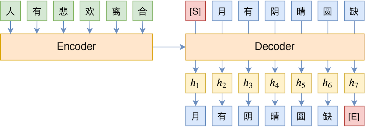
For example, in the figure above, the vector h_3 is only used by Teacher Forcing to predict “cloudy”. In fact, the prediction result of “cloudy” will also affect the predictions of “sunny”, “round”, and “incomplete”. That is to say, h_3 should also be associated with “sunny”, “round”, and “incomplete”, but Teacher Forcing does not explicitly establish this association. Consequently, the model is likely to output only the locally most probable token at each step during decoding, which easily leads to high-frequency “safe” responses or repetitive decoding.

Student Forcing

To improve the model’s “foresight capability,” the most thorough method is to conduct the training phase in the same way as decoding. That is, h_1, h_2, \dots, h_t are predicted recursively just like in the decoding phase, without relying on ground-truth labels. We might call this method Student Forcing. However, the Student Forcing training method brings two serious problems:

First, sacrificing parallelism. For Teacher Forcing, if the Decoder uses a structure like CNN or Transformer, all tokens can be trained in parallel during the training phase (inference is still serial). But with Student Forcing, it is always serial.

Second, extremely difficult convergence. Student Forcing usually requires Gumbel Softmax or Reinforcement Learning to backpropagate gradients. Their training faces severe instability. Generally, Teacher Forcing pre-training is required before using Student Forcing, but even then, it is not particularly stable.

To understand this figuratively, Student Forcing is equivalent to a teacher letting a student explore a complex problem completely independently without step-by-step guidance, only giving a final evaluation of the student’s result. If the student succeeds, it might mean the student’s ability is very strong, but the problem is the lack of the teacher’s “patient guidance,” making the chance of the student “hitting a wall” much higher.

Looking a Few Steps Ahead

Is there a method between Teacher Forcing and Student Forcing? Yes, TeaForN, introduced in this article, is one such method. Its idea is that conventional Teacher Forcing is equivalent to looking ahead 1 step during training, while Student Forcing is equivalent to looking ahead L steps (where L is the target sentence length). If we just look ahead a few more steps (equivalent to seeing N-grams), we can theoretically improve “foresight” without severely sacrificing the model’s parallelism. Its schematic is as follows:

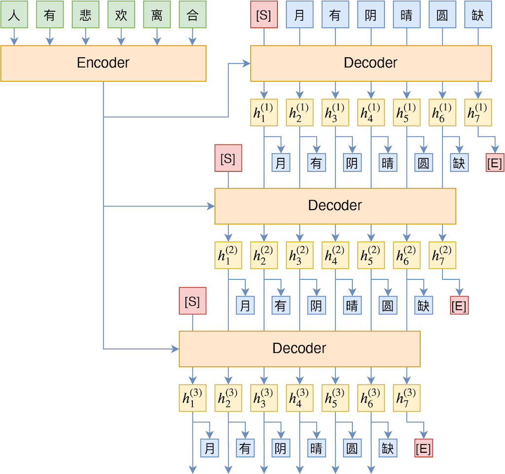
Intuitively, it involves iterating the output results forward multiple times. In this way, the first t-1 tokens are used to predict not just the t-th token, but also the (t+1)-th, (t+2)-th, and so on. For example, in the figure above, we finally use h_6^{(3)} to predict the character “incomplete”. We can see that h_6^{(3)} depends only on the three characters “moon”, “has”, and “cloudy”. Therefore, we can also understand that the vector h_4^{(1)} must simultaneously predict the three characters “sunny”, “round”, and “incomplete”, thereby improving “foresight.”

In Mathematical Terms

Describing this in mathematical language, we can divide the Decoder into two parts: the Embedding layer E and the remaining part M. The Embedding layer is responsible for mapping the input sentence s=[w_0, w_1, w_2, \dots, w_{L-1}] into a sequence of vectors [e_0, e_1, e_2, \dots, e_{L-1}] (where w_0 is a fixed decoding start token, i.e., [S] in the figure above, sometimes denoted as <bos>). This is then handed over to the model M to obtain the vector sequence [h_1, h_2, h_3, \dots, h_L], i.e., = M(E([w_0, w_1, w_2, \dots, w_{L-1}])) Then, the token probability distribution at step t is obtained via p_t = \text{softmax}(Wh_t + b), and finally, -\log p_t[w_t] is used as the loss function for training. This is conventional Teacher Forcing.

One can imagine that the output vector sequence [h_1, h_2, h_3, \dots, h_{L-1}], which is responsible for mapping to the token distribution, is to some extent similar to the Embedding sequence [e_1, e_2, e_3, \dots, e_{L-1}]. If we supplement an e_0 and feed [e_0, h_1, h_2, \dots, h_{L-1}] into the model M for processing again, would that work? That is: \begin{aligned} \left[e_0, e_1, e_2, \dots, e_{L-1}\right] &= E\left(\left[w_0, w_1, w_2, \dots, w_{L-1}\right]\right) \\ \left[h_1^{(1)}, h_2^{(1)}, h_3^{(1)}, \dots, h_L^{(1)}\right] &= M\left(\left[e_0, e_1, e_2, \dots, e_{L-1}\right]\right) \\ \left[h_1^{(2)}, h_2^{(2)}, h_3^{(2)}, \dots, h_L^{(2)}\right] &= M\left(\left[e_0, h_1^{(1)}, h_2^{(1)}, \dots, h_{L-1}^{(1)}\right]\right) \\ \left[h_1^{(3)}, h_2^{(3)}, h_3^{(3)}, \dots, h_L^{(3)}\right] &= M\left(\left[e_0, h_1^{(2)}, h_2^{(2)}, \dots, h_{L-1}^{(2)}\right]\right) \\ &\,\,\vdots \end{aligned} Then, for every h, we calculate the probability distribution p_t^{(i)} = \text{softmax}(Wh_t^{(i)} + b), and finally calculate the cross-entropy and perform a weighted summation: \text{loss} = -\sum_{t=1}^L \sum_{i=1}^N \lambda_i \log p_t^{(i)}[w_t] After training is complete, we only use E and M for conventional decoding operations (such as Beam Search), meaning we only use h_t^{(1)} and do not need h_t^{(2)}, h_t^{(3)}, \dots anymore. This process is the protagonist of this article, TeaForN.

Results, Reflections, and Discussion

As for the experimental results, there is naturally an improvement. Looking at the experimental tables in the original paper, the improvement is more significant when the beam_size is relatively large. Actually, it’s not hard to understand; logically, such processing shouldn’t lead to a decrease in performance at the very least, so it can be considered a “win-win” strategy.

The original paper discusses several points worth debating; let’s look at them here.

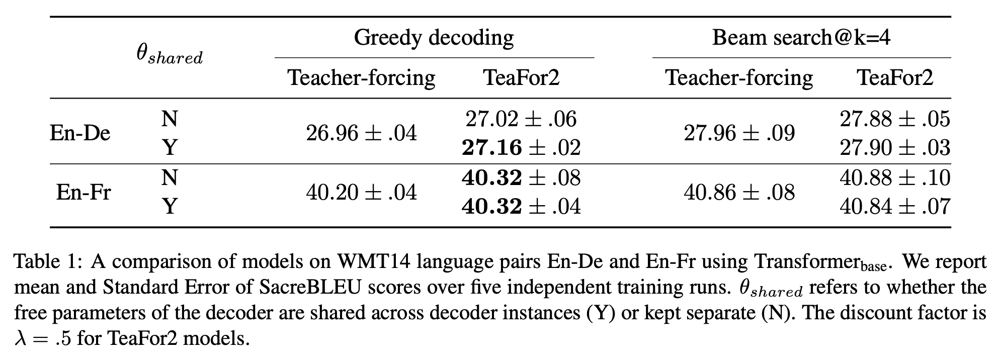
First, should the M used in each iteration step share weights? Intuitively, sharing is better. If weights are not shared, then looking ahead N steps would make the number of parameters nearly N times the original, which doesn’t seem ideal. Of course, it’s best to rely on experiments. The original paper did perform this comparison and confirmed our intuition.

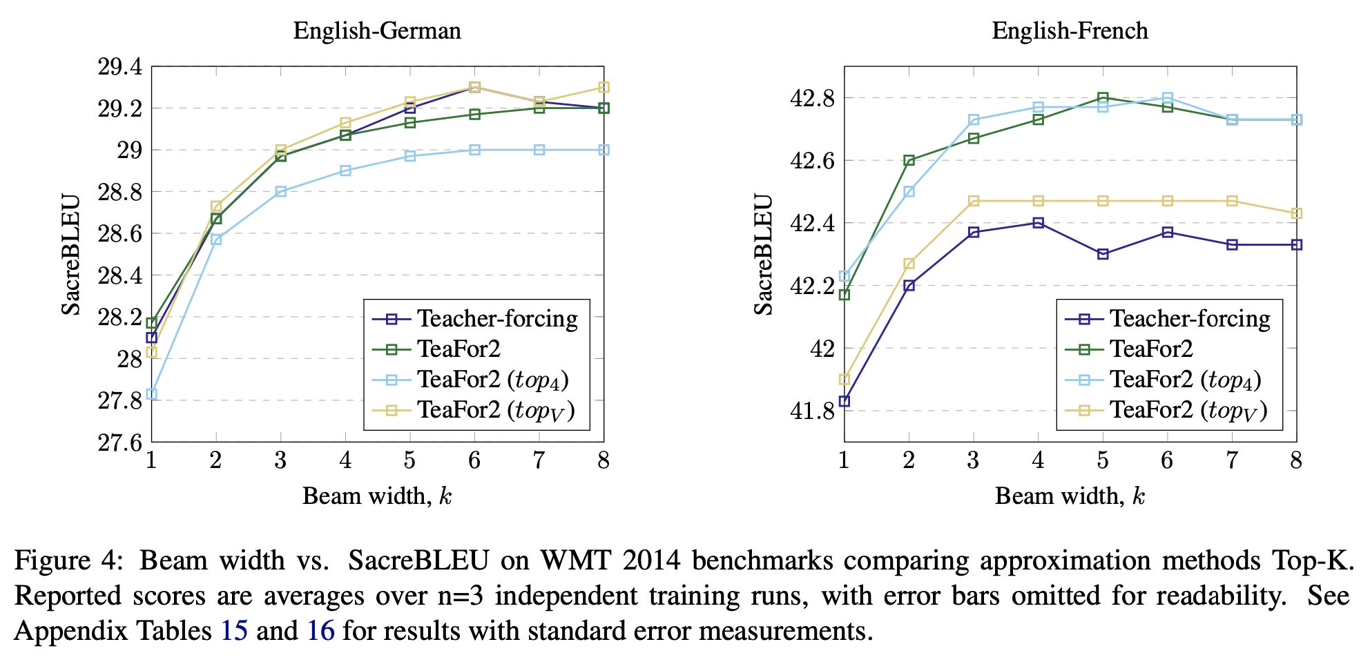
Second, perhaps the main question is: is it really reliable to use [h_1, h_2, h_3, \dots, h_{L-1}] as [e_1, e_2, e_3, \dots, e_{L-1}] during the iteration process? Of course, the experimental results have already shown it is feasible, which is the most convincing argument. However, since h_t is mapped to p_t via an inner product, h_t and e_t might not be similar. If they could be made closer, would the effect be better? The original paper considered the following method: \frac{\sum\limits_{w\in \text{Top}_k(p_t)}p_t[w] e_w}{\sum\limits_{w\in \text{Top}_k(p_t)}p_t[w]} That is, after calculating p_t at each step, take the k tokens with the highest probability and use the weighted average of their Embedding vectors as the input for the next iteration. The original paper experimented with k=4 and k=|V| (vocabulary size), and the results are shown below. Overall, the effect of Top-k is not very stable, and the best cases are similar to directly using h_t, so there’s no need to try others.

Of course, I think it would have been even more perfect if the paper had also compared the effect of simulating sampling via Gumbel Softmax.

Summary

This article shared a new training method proposed by Google called TeaForN. It sits between Teacher Forcing and Student Forcing, can mitigate the model’s Exposure Bias problem, and does not severely sacrifice the parallelism of model training. It is a strategy worth trying. Beyond that, it actually provides a new way of thinking about solving such problems (maintaining parallelism and foresight through iteration), which is quite thought-provoking.

When reposting, please include the original address of this article: https://kexue.fm/archives/7818

For more detailed reposting matters, please refer to: “Scientific Space FAQ”