Some time ago, my company organized a technical sharing session. When it was my turn, everyone wanted me to talk about VAEs. Given that I had previously written a Variational Autoencoder series, I thought it wouldn’t be particularly difficult and agreed. However, upon closer reflection, I found myself in a dilemma: how should I present it?
Regarding VAEs, I have previously written two systematic introductions: "Variational Autoencoders (Part 1): So That’s How It Is" and "Variational Autoencoders (Part 2): From a Bayesian Perspective". The latter is a pure probabilistic derivation, which might not be very meaningful or understandable for those not doing theoretical research. The former, while more accessible, is also not entirely ideal because it approaches the topic from the perspective of generative models and doesn’t clearly explain "why we need VAE" (to put it bluntly, VAEs can yield generative models, but VAEs are not necessarily intended only for generative models), and its overall style isn’t particularly friendly.
I thought about it and realized that for most readers who don’t know VAEs but want to use them, they likely only want a rough understanding of the VAE form and answers to questions like "What is the role of VAE?", "What is the difference between VAE and AE?", and "In what scenarios is VAE needed?". Neither of the above articles satisfies these needs well. Therefore, I tried to conceive a geometric picture of VAE, attempting to describe its key characteristics from a geometric perspective, which I would like to share with you here.
Autoencoder
We start with the Autoencoder (AE). The original intention of an autoencoder is data dimensionality reduction. Assuming the original feature x has a dimension that is too high, we hope to encode it into a low-dimensional feature vector z=E(x) through an encoder E. The principle of encoding is to retain as much original information as possible. Therefore, we train a decoder D, hoping to reconstruct the original information through z, i.e., x \approx D(E(x)). Its optimization objective is generally: E,D = \mathop{\text{argmin}}_{E,D}\mathbb{E}_{x\sim \mathcal{D}}\big[\Vert x - D(E(x))\Vert^2\big] The corresponding diagram is as follows:

Encoding Space
If every sample can be reconstructed well, we can treat z as an equivalent representation of x. In other words, studying z well is equivalent to studying x well. Now, we encode every x into its corresponding feature vector z, and then we care about one question: What does the space covered by these z "look like"?
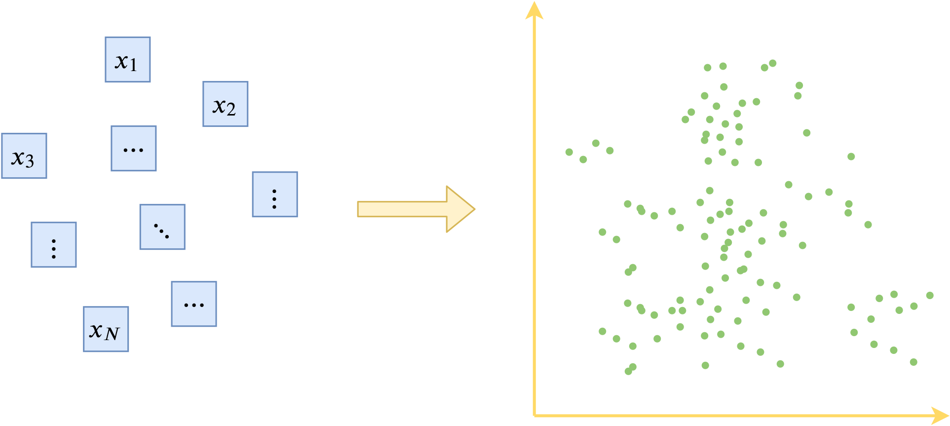
Why care about this? Because we can have many different encoding methods, and the feature vectors obtained by different encoding methods vary in quality. From "what the encoding space looks like," we can roughly see the quality of the feature vectors. For example, here are four simulation diagrams of different distribution shapes of encoding vectors:

The vector distribution in the first image has no special shape and is quite scattered, indicating that the encoding space is not particularly regular. In the second image, the vectors are concentrated on a line, indicating redundancy between the dimensions of the encoding vectors. The third image is a ring, indicating that there are no corresponding real samples near the center of the circle. The fourth image is a circle, indicating that it covers a continuous space quite regularly. Looking at the four images, we consider the vector distribution shape depicted in the last image to be the most ideal: regular, non-redundant, and continuous. This means that if we learn from a subset of samples, it is easy to generalize to unknown new samples. Because we know the encoding space is regular and continuous, we know that the "gaps" between the encoding vectors of training samples (the blank parts between two points in the figure) actually correspond to unknown real samples. Therefore, by handling the knowns well, it is very likely that the unknowns are also handled well.
From Point to Surface
In general, we are concerned with the following questions regarding the encoding space:
What kind of region do all encoding vectors cover?
Are there unknown real samples corresponding to the vectors in the blank spaces?
Are there any "outlier" vectors?
Is there a way to make the encoding space more regular?
Conventional autoencoders have difficulty answering these questions because they lack specific constraints. Thus, the Variational Autoencoder emerged. From an encoding perspective, its goals are: 1. To make the encoding space more regular; 2. To make the encoding vectors more compact. To achieve this, the Variational Autoencoder first introduces the posterior distribution p(z|x).
For readers who do not want to delve into probabilistic language, how should we understand the posterior distribution p(z|x)? Intuitively, we can understand the posterior distribution as an "ellipse." Originally, each sample corresponded to an encoding vector, which is a point in the encoding space. After introducing the posterior distribution, it is as if each sample x now corresponds to an "ellipse." We just said we hope the encoding vectors are more "compact," but theoretically, no matter how many "points" there are, they cannot cover a "surface." However, if we use "surfaces" to cover a "surface," it becomes easier to cover the target. This is one of the main changes made by the Variational Autoencoder.
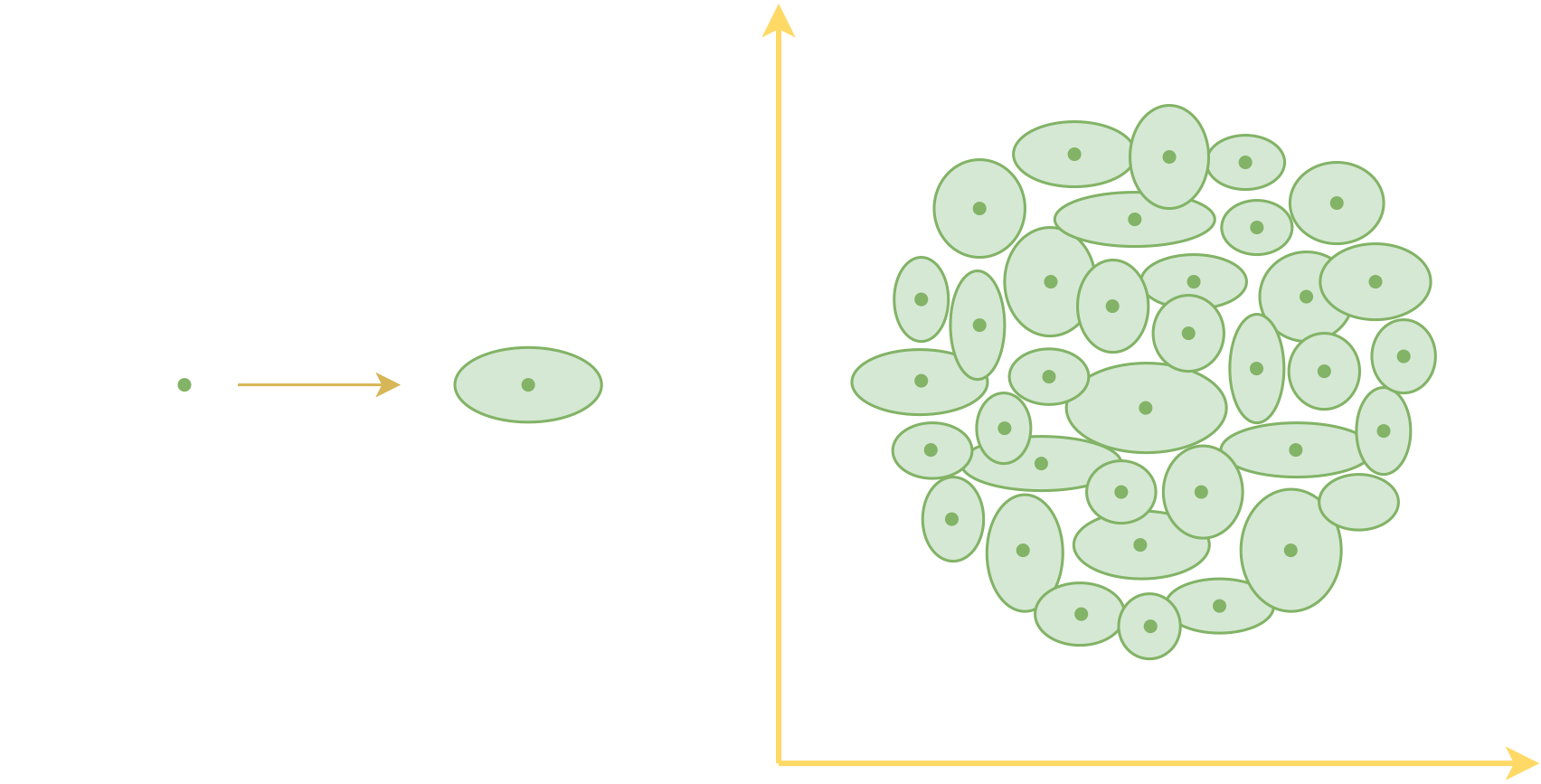
Readers might ask, why must it be an ellipse? Can it be a rectangle or other shapes? Returning to probabilistic language, an ellipse corresponds to the "assumption that p(z|x) is a Gaussian distribution with independent components." From a probabilistic perspective, the Gaussian distribution is a class of probability distributions that is relatively easy to handle. Therefore, we use the Gaussian distribution, which corresponds to an ellipse. Other shapes would correspond to other distributions; for example, a rectangle could correspond to a uniform distribution, but calculating the KL divergence later would be more troublesome, so it is generally not used.
Sampling and Reconstruction
Now each sample x corresponds to an "ellipse." To determine an "ellipse," two pieces of information are needed: the center of the ellipse and the axis lengths. Each of these forms a vector, and these vectors depend on the sample x; we denote them as \mu(x) and \sigma(x). Since the entire ellipse corresponds to the sample x, we require that any point within the ellipse can reconstruct x. Therefore, the training objective is: \mu,\sigma,D = \mathop{\text{argmin}}_{\mu,\sigma,D}\mathbb{E}_{x\sim \mathcal{D}}\big[\Vert x - D(\mu(x) + \varepsilon\otimes \sigma(x))\Vert^2\big],\quad \varepsilon\sim \mathcal{N}(0, 1) where \mathcal{D} is the training data and \mathcal{N}(0, 1) is the standard normal distribution, which we can understand as a unit circle. That is to say, we first sample \varepsilon from the unit circle, and then transform it into a point within the ellipse with "center \mu(x) and axis lengths \sigma(x)" through the translation and scaling transformation \mu(x) + \varepsilon\otimes \sigma(x). This process is the so-called "Reparameterization."
Here, \mu(x) actually corresponds to the encoder E(x) in the autoencoder, and \sigma(x) corresponds to the range it can generalize to.
Space Regularization
Finally, while the "ellipse" can "make the encoding vectors more compact," it cannot yet "make the encoding space more regular." Now we hope that the encoding vectors satisfy a standard normal distribution (which can be understood as a unit circle), meaning that the space covered by all ellipses forms a unit circle.
To this end, we hope that each ellipse can move closer to the unit circle. The center of the unit circle is 0 and the radius is 1, so a basic idea is to introduce a regularization term: \mathbb{E}_{x\sim \mathcal{D}}\big[\Vert \mu(x) - 0\Vert^2 + \Vert \sigma(x) - 1\Vert^2\big] In fact, combining these first two loss terms is already very close to the standard Variational Autoencoder. The standard Variational Autoencoder uses a slightly more complex but functionally similar regularization term: \mathbb{E}_{x\sim \mathcal{D}}\left[\sum_{i=1}^d \frac{1}{2}\Big(\mu_{i}^2(x) + \sigma_{i}^2(x) - \log \sigma_{i}^2(x) - 1\Big)\right] This regularization term originates from the KL divergence between two Gaussian distributions, so it is also commonly called the "KL divergence term."
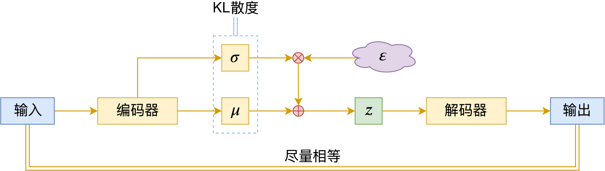
Combining the two objectives, we get the final Variational Autoencoder: \Vert x - D(\mu(x) + \varepsilon\otimes \sigma(x))\Vert^2 + \sum_{i=1}^d \frac{1}{2}\Big(\mu_{i}^2(x) + \sigma_{i}^2(x) - \log \sigma_{i}^2(x) - 1\Big), \quad \varepsilon\sim \mathcal{N}(0, 1)
Conclusion
This article introduced an understanding of the Variational Autoencoder (VAE) from the perspective of geometric analogy. In this view, the goal of the VAE is to make the encoding vectors more compact and to regularize the encoding distribution into a standard normal distribution (unit circle).
In this way, VAE achieves two effects: 1. By randomly sampling a vector from the standard Gaussian distribution (unit circle), the decoder can produce a real sample, thus realizing a generative model; 2. Due to the compactness of the encoding space and the noise added to the encoding vectors during training, the various components of the encoding vector can achieve a certain degree of decoupling and be endowed with certain linear arithmetic properties.
The geometric perspective allows us to quickly grasp the key characteristics of Variational Autoencoders and reduces the difficulty of entry, but it also has certain imprecisions. If there are any inaccuracies, I hope readers will understand and point them out.
When reposting, please include the original address of this article: https://kexue.fm/archives/7725
For more detailed reposting matters, please refer to: "Scientific Space FAQ"