When training a model, do we need the loss function to be trained all the way to zero? Obviously not. Generally speaking, we use the training set to train the model, but we hope that the loss on the validation set is as small as possible. Normally, after the training loss drops to a certain value, the validation loss will start to rise; therefore, it is unnecessary to reduce the training loss to zero.
That being the case, can we do something else to improve model performance after a certain threshold has been reached? The ICML 2020 paper "Do We Need Zero Training Loss After Achieving Zero Training Error?" answers this question. However, the paper’s answer is limited to the level of "what it is" and does not describe "why" very well. Furthermore, after reading the interpretation by the expert kid on Zhihu, I still couldn’t find the answer I wanted. Therefore, I analyzed it myself and recorded it here.
Description of the Idea
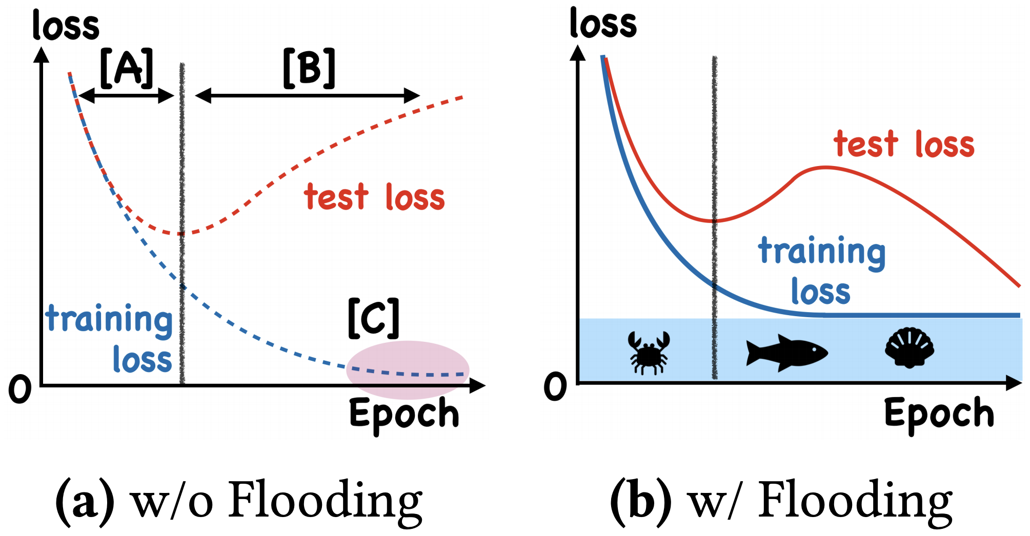
The solution provided by the paper is very simple. Suppose the original loss function is \mathcal{L}(\theta); it is now changed to \tilde{\mathcal{L}}(\theta): \tilde{\mathcal{L}}(\theta)=|\mathcal{L}(\theta) - b|+b where b is a pre-set threshold. When \mathcal{L}(\theta) > b, \tilde{\mathcal{L}}(\theta)=\mathcal{L}(\theta), which is just performing ordinary gradient descent. When \mathcal{L}(\theta) < b, \tilde{\mathcal{L}}(\theta)=2b-\mathcal{L}(\theta). Notice that the sign of the loss function has changed, so at this point, it is gradient ascent. Therefore, in general, b is used as a threshold; when the loss is below the threshold, we actually want the loss function to increase. The paper calls this modification "Flooding."
What is the effect of doing this? The paper shows that in some tasks, after the training loss is processed this way, the validation loss can exhibit "Double Descent," as shown in the figure below:
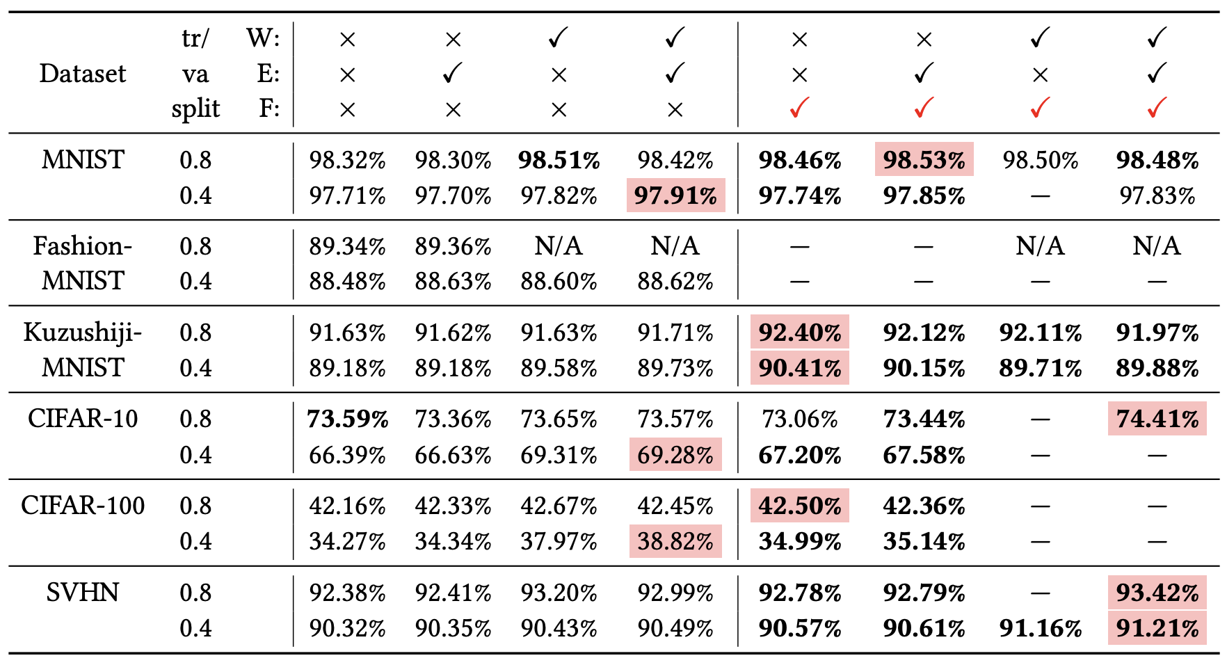
Simply put, the final performance on the validation set may be better. The experimental results from the original paper are as follows:
Personal Analysis
How can we explain this method? One can imagine that after the loss function reaches b, the training process roughly alternates between gradient descent and gradient ascent. Intuitively, it might seem that one step up and one step down would just cancel each other out. Is this really the case? Let’s calculate and see. Suppose we take one step down followed by one step up, with a learning rate \varepsilon: \begin{aligned} &\theta_n = \theta_{n-1} - \varepsilon g(\theta_{n-1})\\ &\theta_{n+1} = \theta_n + \varepsilon g(\theta_n) \end{aligned} where g(\theta)=\nabla_{\theta}\mathcal{L}(\theta). Now we have: \begin{aligned} \theta_{n+1} =&\, \theta_{n-1} - \varepsilon g(\theta_{n-1}) + \varepsilon g\big(\theta_{n-1} - \varepsilon g(\theta_{n-1})\big)\\ \approx&\,\theta_{n-1} - \varepsilon g(\theta_{n-1}) + \varepsilon \big(g(\theta_{n-1}) - \varepsilon \nabla_{\theta} g(\theta_{n-1}) g(\theta_{n-1})\big)\\ =&\,\theta_{n-1} - \frac{\varepsilon^2}{2}\nabla_{\theta}\Vert g(\theta_{n-1})\Vert^2 \end{aligned} Here, \approx denotes the use of a Taylor expansion to approximate the loss function.
The final result is equivalent to gradient descent with a learning rate of \frac{\varepsilon^2}{2} on a loss function that is the gradient penalty \Vert g(\theta)\Vert^2=\Vert\nabla_{\theta}\mathcal{L}(\theta)\Vert^2. Even better, if we change it to "ascent first then descent," the expression remains the same (this reminds me of the story of "raising the price by 10% then lowering it by 10%" versus "lowering the price by 10% then raising it by 10%"). Therefore, on average, the modification of the loss function by Flooding is equivalent to minimizing \Vert\nabla_{\theta}\mathcal{L}(\theta)\Vert^2 after ensuring the loss function is small enough. This pushes the parameters toward a flatter region, which usually improves generalization performance (better resistance to perturbations). Thus, this explains to some extent why Flooding works.
In essence, this is not much different from adding random perturbations to parameters or adversarial training, except that here the perturbation is added only after ensuring the loss is small enough. Readers can refer to "Generalization: From Random Noise, Gradient Penalty to Virtual Adversarial Training" for related content, or the "Regularization" section in Chapter 7 of Part II of the "Bible" Deep Learning.
Further Brainstorming
Readers interested in using this method might struggle with the choice of b. However, I have another idea: b simply determines when to start alternating training. What if we use different learning rates for alternating training from the very beginning? That is, execute the following from start to finish: \begin{aligned} &\theta_n = \theta_{n-1} - \varepsilon_1 g(\theta_{n-1})\\ &\theta_{n+1} = \theta_n + \varepsilon_2 g(\theta_n) \end{aligned} where \varepsilon_1 > \varepsilon_2. This way, we remove b (though we introduce the choice of \varepsilon_1/\varepsilon_2; there is no free lunch). Repeating the above approximate expansion, we get: \begin{aligned} \theta_{n+1} \approx&\, \theta_{n-1} - (\varepsilon_1 - \varepsilon_2) g(\theta_{n-1}) - \frac{\varepsilon_1\varepsilon_2}{2}\nabla_{\theta}\Vert g(\theta_{n-1})\Vert^2\\ =&\,\theta_{n-1} - (\varepsilon_1 - \varepsilon_2)\nabla_{\theta}\left[\mathcal{L}(\theta_{n-1}) + \frac{\varepsilon_1\varepsilon_2}{2(\varepsilon_1 - \varepsilon_2)}\Vert \nabla_{\theta}\mathcal{L}(\theta_{n-1})\Vert^2\right] \end{aligned} This is equivalent to optimizing the loss function \mathcal{L}(\theta) + \frac{\varepsilon_1\varepsilon_2}{2(\varepsilon_1 - \varepsilon_2)}\Vert\nabla_{\theta}\mathcal{L}(\theta)\Vert^2 with a learning rate of \varepsilon_1 - \varepsilon_2 from the very beginning. In other words, the gradient penalty is added from the start. Can this improve the model’s generalization performance? I tried it briefly; in some cases, there is a slight improvement, and generally, there are no negative effects. Overall, it is not as good as directly adding a gradient penalty yourself, so I do not recommend doing it this way.
Note: Reader @xx205 provided the reference "Backstitch: Counteracting Finite-sample Bias via Negative Steps", which points out that this approach is effective in speech recognition. Therefore, my statement above may not be entirely complete; readers should test and discern for themselves. Thanks again to reader @xx205 for the information.
Conclusion
This article briefly introduced the training strategy of "gradient ascent after a certain point" proposed in an ICML 2020 paper and provided my own derivation and understanding. The results show that it is equivalent to a gradient penalty on the parameters, and gradient penalty is one of the common regularization methods.
When reposting, please include the original link: https://kexue.fm/archives/7643
For more detailed reposting matters, please refer to: "Scientific Space FAQ"