Mitigating Class Imbalance via Mutual Information

Problem Description

We are primarily concerned with single-label multi-class classification. Suppose there are K candidate categories 1, 2, \dots, K. The training data is (x, y) \sim \mathcal{D}, and the modeled distribution is p_{\theta}(y|x). Our optimization goal is maximum likelihood, or equivalently, minimizing cross-entropy: \mathop{\text{argmin}}_{\theta}\,\mathbb{E}_{(x,y)\sim\mathcal{D}}[-\log p_{\theta}(y|x)] Typically, the last step of the probabilistic models we build is a softmax. Assuming the result before softmax is f(x;\theta) (i.e., logits), then: -\log p_{\theta}(y|x)=-\log \frac{e^{f_y(x;\theta)}}{\sum\limits_{i=1}^K e^{f_i(x;\theta)}}=\log\left[1 + \sum_{i\neq y}e^{f_i(x;\theta) - f_y(x;\theta)}\right] \label{eq:loss-1} Class imbalance refers to the situation where some categories have a particularly large number of samples, much like "20% of the people hold 80% of the wealth." The remaining categories are numerous, but their total sample count is small. If sorted from high to low frequency, it looks like a long "tail," hence the name long-tail phenomenon. In this case, when we sample a batch during training, there is little chance of sampling low-frequency categories, making it easy for the model to ignore them. However, during evaluation, we usually care more about the recognition performance of these low-frequency categories. This is the contradiction.

Common Approaches

Common strategies you might have heard of generally fall into three directions:

1. Data-level: Using techniques like oversampling or undersampling to make the categories within each batch more balanced.

2. Loss-level: A classic approach is to divide the loss of a sample from category y by the frequency of that category p(y).

3. Result-level: Adjusting the predictions of a normally trained model during the inference phase to favor low-frequency categories. For example, if positive samples are much fewer than negative ones, we might treat all predictions greater than 0.2 (instead of 0.5) as positive.

The original Google paper lists many references for these three directions. Interested readers can read the original paper. Additionally, the Zhihu article "Long-Tailed Classification (2) Latest Research on Classification under Long-Tailed Distribution" also introduces this problem and is worth a read.

Learning Mutual Information

Recall, how do we determine that a classification problem is imbalanced? Obviously, the general approach is to calculate the frequency p(y) of each category from the entire training set and find that p(y) is concentrated in a few categories. Therefore, the key to solving the class imbalance problem is how to integrate this prior knowledge p(y) into the model.

When I was previously conceiving word vector models (such as in the article "A More Unique Word Vector Model (II): Modeling Language"), I emphasized that compared to fitting conditional probability, if a model can directly fit mutual information, it will learn more essential knowledge, because mutual information is the indicator that reveals core associations. However, fitting mutual information is not easy to train. What is easy to train is conditional probability, using cross-entropy -\log p_{\theta}(y|x) directly. So, an ideal idea is: How can we make the model still use cross-entropy as the loss, but essentially fit mutual information?

In Equation [eq:loss-1], we modeled: p_{\theta}(y|x)=\frac{e^{f_y(x;\theta)}}{\sum\limits_{i=1}^K e^{f_i(x;\theta)}} Now we change to modeling mutual information, which means we hope: \log \frac{p_{\theta}(y|x)}{p(y)}\sim f_y(x;\theta)\quad \Leftrightarrow\quad \log p_{\theta}(y|x)\sim f_y(x;\theta) + \log p(y) Performing softmax normalization according to the form on the right, we get p_{\theta}(y|x)=\frac{e^{f_y(x;\theta)+\log p(y)}}{\sum\limits_{i=1}^K e^{f_i(x;\theta)+\log p(i)}}, or written in loss form: -\log p_{\theta}(y|x)=-\log \frac{e^{f_y(x;\theta)+\log p(y)}}{\sum\limits_{i=1}^K e^{f_i(x;\theta)+\log p(i)}}=\log\left[1 + \sum_{i\neq y}\frac{p(i)}{p(y)}e^{f_i(x;\theta) - f_y(x;\theta)}\right] \label{eq:loss-2} The original paper calls this the logit adjustment loss. For a more generalized version, one can add a scaling factor \tau: -\log p_{\theta}(y|x)=-\log \frac{e^{f_y(x;\theta)+\tau\log p(y)}}{\sum\limits_{i=1}^K e^{f_i(x;\theta)+\tau\log p(i)}}=\log\left[1 + \sum_{i\neq y}\left(\frac{p(i)}{p(y)}\right)^{\tau}e^{f_i(x;\theta) - f_y(x;\theta)}\right] \label{eq:loss-3} In general, the effect of \tau=1 is already close to optimal. If the last layer of f_y(x;\theta) has a bias term, the simplest implementation is to initialize the bias term to \tau\log p(y). It can also be written in the loss function:

import numpy as np
import keras.backend as K

def categorical_crossentropy_with_prior(y_true, y_pred, tau=1.0):
    """Cross-entropy with prior distribution
    Note: y_pred should not have softmax applied
    """
    prior = xxxxxx  # Define your own prior, shape [num_classes]
    log_prior = K.constant(np.log(prior + 1e-8))
    for _ in range(K.ndim(y_pred) - 1):
        log_prior = K.expand_dims(log_prior, 0)
    y_pred = y_pred + tau * log_prior
    return K.categorical_crossentropy(y_true, y_pred, from_logits=True)

def sparse_categorical_crossentropy_with_prior(y_true, y_pred, tau=1.0):
    """Sparse cross-entropy with prior distribution
    Note: y_pred should not have softmax applied
    """
    prior = xxxxxx  # Define your own prior, shape [num_classes]
    log_prior = K.constant(np.log(prior + 1e-8))
    for _ in range(K.ndim(y_pred) - 1):
        log_prior = K.expand_dims(log_prior, 0)
    y_pred = y_pred + tau * log_prior
    return K.sparse_categorical_crossentropy(y_true, y_pred, from_logits=True)

Analysis of Results

Clearly, logit adjustment loss belongs to the category of loss adjustment schemes. The difference is that it adjusts weights inside the \log, whereas conventional approaches adjust outside the \log. As for its benefits, they are the benefits of mutual information: mutual information reveals truly important associations. By adding the bias of the prior distribution to the logits, the model can achieve the goal of "solving what can be solved by the prior using the prior, and letting the model solve only the essential parts that the prior cannot solve."

In the prediction phase, we can formulate different prediction schemes based on different evaluation metrics. From "Random Talk on Function Smoothing: Differentiable Approximation of Non-differentiable Functions", we know that for overall accuracy, we have the approximation: \text{Overall Accuracy} \approx \frac{1}{N}\sum_{i=1}^N p_{\theta}(y_i|x_i) where \{(x_i,y_i)\}_{i=1}^N is the validation set. So if we do not consider class imbalance and pursue higher overall accuracy, we can directly output the category with the largest p_{\theta}(y|x) for each x. However, if we want the accuracy of each class to be as high as possible, we rewrite the above formula as: \text{Overall Accuracy} \approx \frac{1}{N}\sum_{i=1}^N \frac{p_{\theta}(y_i|x_i)}{p(y_i)}\times p(y_i)=\sum_{y=1}^K p(y)\left(\frac{1}{N}\sum_{x_i\in\Omega_y} \frac{p_{\theta}(y|x_i)}{p(y)}\right) where \Omega_y=\{x_i|y_i=y,i=1,2,\dots,N\} is the set of x with label y. The right side of the equation essentially groups terms with the same y together. We know that "Overall Accuracy = weighted average of the accuracy of each class," and the above formula has exactly the same form. Therefore, the term in the parentheses \frac{1}{N}\sum\limits_{x_i\in\Omega_y} \frac{p_{\theta}(y|x_i)}{p(y)} is an approximation of the "accuracy of each class." Thus, if we want the accuracy of each class to be as high as possible, we should output the category that maximizes \frac{p_{\theta}(y|x)}{p(y)} (unweighted). Combining this with the form of p_{\theta}(y|x), we have the conclusion: y^{*}=\left\{\begin{aligned}&\mathop{\text{argmax}}\limits_y\, f_y(x;\theta)+\tau\log p(y),\quad(\text{Pursuing overall accuracy})\\ &\mathop{\text{argmax}}\limits_y\, f_y(x;\theta),\quad(\text{Hoping for uniform accuracy across classes}) \end{aligned}\right. The first case is outputting the one with the maximum conditional probability, while the second is outputting the one with the maximum mutual information. Choose according to specific needs.

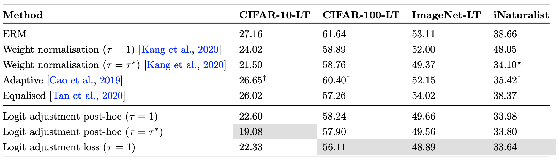
For detailed experimental results, please refer to the paper. In short, they are surprisingly good:

Summary

This article briefly introduced a class imbalance handling method based on the idea of mutual information. I had conceived this scheme before but did not investigate it deeply. A recent paper from Google proposed the same method, so I have recorded and analyzed it here. Finally, the experimental results provided by Google show that this method can reach SOTA levels.

Original address: https://kexue.fm/archives/7615

For more details on reprinting, please refer to: "Scientific Space FAQ"