This article introduces a visualization method for neural networks: Integrated Gradients. It was first proposed in the paper "Gradients of Counterfactuals" and later reintroduced in "Axiomatic Attribution for Deep Networks". The authors of both papers are the same, and the content is largely similar, though the latter is relatively easier to understand. If you intend to read the original papers, I recommend starting with the second one. Of course, this work dates back to 2016–2017; "novel" refers to the innovative and interesting nature of its approach rather than a very recent publication date.
In simple terms, visualization means that for a given input x and a model F(x), we find a way to identify which components of x have a significant impact on the model’s decision, or to rank the importance of each component of x. In professional terminology, this is called "attribution." A naive approach is to directly use the gradient \nabla_x F(x) as an indicator of the importance of each component of x, and Integrated Gradients is an improvement upon this. However, I believe many articles introducing Integrated Gradients (including the original papers) are too "stiff" (formalistic) and do not effectively highlight the fundamental reason why Integrated Gradients is more effective than naive gradients. This article attempts to introduce the Integrated Gradients method using my own perspective.
Naive Gradients
First, let’s look at gradient-based methods, which are essentially based on the Taylor expansion: F(x+\Delta x) - F(x) \approx \langle\nabla_x F(x), \Delta x\rangle = \sum_i [\nabla_x F(x)]_i \Delta x_i \label{eq:g} We know that \nabla_x F(x) is a vector of the same size as x. Here, [\nabla_x F(x)]_i is its i-th component. For a fixed magnitude of \Delta x_i, the larger the absolute value of [\nabla_x F(x)]_i, the greater the change in F(x+\Delta x) relative to F(x). That is to say:
[\nabla_x F(x)]_i measures the sensitivity of the model to the i-th component of the input, so we use |[\nabla_x F(x)]_i| as the importance indicator for the i-th component.
This approach is simple and direct. It has been described in papers such as "How to Explain Individual Classification Decisions" and "Deep Inside Convolutional Networks: Visualising Image Classification Models and Saliency Maps". In many cases, it can indeed successfully explain some prediction results, but it has obvious drawbacks. Many articles mention the issue of saturation regions; once the model enters a saturation region (a classic example being the negative half-axis of ReLU), the gradient becomes 0, and it fails to reveal any useful information.
From a practical standpoint, this understanding is reasonable, but I believe it is not profound enough. As seen in the previous article "A Brief Discussion on Adversarial Training: Significance, Methods, and Reflections", the goal of adversarial training can be understood as pushing \|\nabla_x F(x)\|^2 \to 0. This implies that gradients can be "manipulated"; even without affecting the model’s prediction accuracy, we can make the gradients as close to 0 as possible. Therefore, returning to the theme of this article: [\nabla_x F(x)]_i indeed measures the sensitivity of the model to the i-th component of the input, but sensitivity is not a good measure of importance.
Integrated Gradients
Given the aforementioned shortcomings of using gradients directly, several improvements have been proposed, such as LRP and DeepLift. However, relatively speaking, I find the improvement offered by Integrated Gradients to be more concise and elegant.
Reference Background
First, we need to understand the original problem from a different angle: Our goal is to find the important components, but this importance should not be absolute; it should be relative. For example, if we want to find recently popular buzzwords, we cannot look at word frequency alone; otherwise, we would just find stop words like "the" or "is." We should prepare a "reference" frequency table calculated from a balanced corpus and then compare the difference in frequency rather than the absolute value. This tells us that to measure the importance of each component of x, we also need a "reference background" \bar{x}.
In many scenarios, we can simply let \bar{x}=0, but this is not necessarily optimal. For instance, we could choose \bar{x} to be the mean of all training samples. We expect F(\bar{x}) to yield a relatively trivial prediction result; for a classification model, the prediction for \bar{x} should have balanced probabilities for each class. Thus, we consider F(\bar{x}) - F(x), which we can imagine as the cost of moving from x to \bar{x}.
If we still use the approximate expansion [eq:g], we get: F(\bar{x}) - F(x) \approx \sum_i [\nabla_x F(x)]_i [\bar{x} - x]_i \label{eq:g2} For the above equation, we can have a new interpretation:
The total cost of moving from x to \bar{x} is F(\bar{x}) - F(x), which is the sum of the costs of each component. The cost of each component is approximately [\nabla_x F(x)]_i [\bar{x} - x]_i, so we can use |[\nabla_x F(x)]_i [\bar{x} - x]_i| as the importance indicator for the i-th component.
Of course, whether it is [\nabla_x F(x)]_i or |[\nabla_x F(x)]_i [\bar{x} - x]_i|, their mathematical flaws are the same (gradient vanishing), but the corresponding explanations are different. As mentioned before, the flaw of [\nabla_x F(x)]_i stems from "sensitivity not being a good measure of importance," whereas throughout the reasoning in this section, the flaw of |[\nabla_x F(x)]_i [\bar{x} - x]_i| is simply because "equation [eq:g2] is only approximately true," but the overall logical reasoning is sound.
Integral Identity
Often, a new explanation brings a new perspective, which in turn inspires new improvements. For example, the previous analysis of the flaw stated that "|[\nabla_x F(x)]_i [\bar{x} - x]_i| is not good enough because equation [eq:g2] is not accurate enough." If we can find a similar expression that is exactly equal, we can solve this problem. Integrated Gradients finds exactly such an expression: let \gamma(\alpha), \alpha \in [0,1] represent a parametric curve connecting x and \bar{x}, where \gamma(0)=x and \gamma(1)=\bar{x}. Then we have: \begin{aligned} F(\bar{x})-F(x) &= F(\gamma(1))-F(\gamma(0))\\ &= \int_0^1 \frac{dF(\gamma(\alpha))}{d\alpha}d\alpha\\ &= \int_0^1 \left\langle\nabla_{\gamma} F(\gamma(\alpha)), \gamma'(\alpha)\right\rangle d\alpha\\ &= \sum_i \int_0^1 \left[\nabla_{\gamma} F(\gamma(\alpha))\right]_i \left[\gamma'(\alpha)\right]_i d\alpha \end{aligned} \label{eq:g3} As we can see, equation [eq:g3] has the same form as [eq:g2], but replaces [\nabla_x F(x)]_i [\bar{x} - x]_i with \int_0^1 \left[\nabla_{\gamma} F(\gamma(\alpha))\right]_i \left[\gamma'(\alpha)\right]_i d\alpha. Since equation [eq:g3] is an exact integral identity, Integrated Gradients proposes using: \left|\int_0^1 \left[\nabla_{\gamma} F(\gamma(\alpha))\right]_i \left[\gamma'(\alpha)\right]_i d\alpha\right| \label{eq:ig-1} as the importance measure for the i-th component. The simplest solution is naturally to take \gamma(\alpha) as the straight line between the two points, i.e., \gamma(\alpha) = (1 - \alpha) x + \alpha \bar{x} In this case, Integrated Gradients is specified as: \left|\left[\int_0^1 \nabla_{\gamma} F(\gamma(\alpha))\big|_{\gamma(\alpha) = (1 - \alpha) x + \alpha \bar{x}}d\alpha\right]_i \left[\bar{x}-x\right]_i\right| \label{eq:ig-2} So, compared to |[\nabla_x F(x)]_i [\bar{x} - x]_i|, it replaces \nabla_x F(x) with the integral of the gradient \int_0^1 \nabla_{\gamma} F(\gamma(\alpha))\big|_{\gamma(\alpha) = (1 - \alpha) x + \alpha \bar{x}}d\alpha, which is the average gradient of every point on the line from x to \bar{x}. Intuitively, because it considers the gradients of all points along the path, it is no longer limited by the gradient being zero at a single point.
If readers look at the two original papers on Integrated Gradients, they will find that the introduction in the original papers is reversed: they first present equation [eq:ig-2] somewhat out of the blue, then prove it satisfies two somewhat arbitrary properties (sensitivity and implementation invariance), and finally prove it satisfies equation [eq:g3]. In short, they take the reader on a long journey without clearly stating the fundamental reason why it is a better measure of importance—everyone is based on the decomposition of F(\bar{x}) - F(x), and equation [eq:g3] is more accurate than equation [eq:g2].
Discrete Approximation
Finally, how do we calculate this integral form? Deep learning frameworks don’t have a built-in function for integration. Actually, it’s simple: according to the "approximation-limit" definition of an integral, we can directly use a discrete approximation. Taking equation [eq:ig-2] as an example, it is approximated by: \left|\left[\frac{1}{n}\sum_{k=1}^n\Big(\nabla_{\gamma} F(\gamma(\alpha))\big|_{\gamma(\alpha) = (1 - \alpha) x + \alpha \bar{x}, \alpha=k/n}\Big)\right]_i \left[\bar{x}-x\right]_i\right| So, as said before, the essence is the "average of the gradients at every point on the straight line from x to \bar{x}," which works better than the gradient at a single point.
Experimental Results
Having covered the theory, let’s look at the experimental results.
Original Results
Original paper implementation: https://github.com/ankurtaly/Integrated-Gradients
Below are some result images from the original paper:


Personal Implementation
Although the Keras official website has provided a reference implementation (see here), the code is quite long and tiring to read. I have implemented one myself using Keras based on my own understanding and applied it to NLP. The specific code can be found at "task_sentiment_integrated_gradients.py". The current code is just a simple demo; readers are welcome to derive more powerful code based on it.
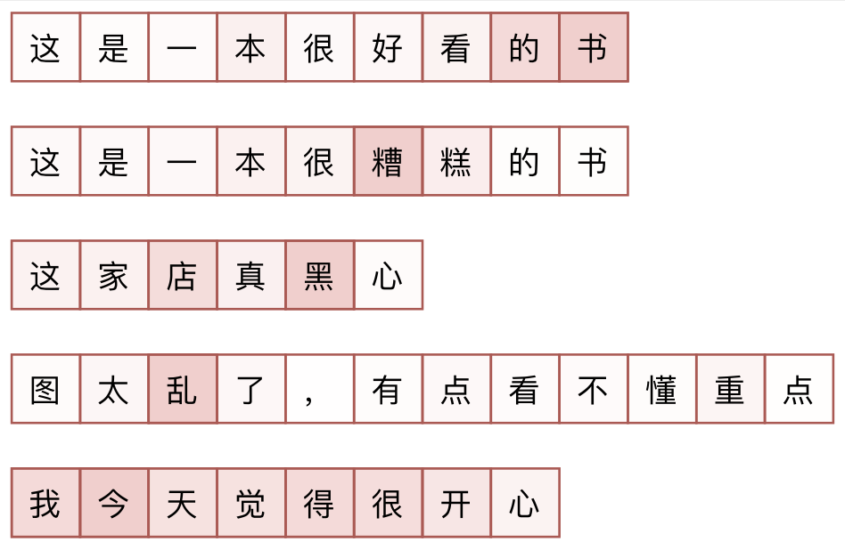
In the figure above, I show the results for several samples (the model’s sentiment label predictions for these samples are all correct). From this, we can infer the principle by which the original model performs sentiment classification. We can see that for negative samples, Integrated Gradients can reasonably locate the negative words in the sentence. However, for positive samples, even if the grammatical structure is the same as the negative samples, it fails to locate the positive words. This phenomenon suggests that the original model’s approach to sentiment classification might be "negative detection"—that is, it primarily detects negative emotions, and if no negative emotion is detected, it is regarded as a positive sample. This is likely a result of not having "neutral" samples for training.
Conclusion
This article introduced a neural network visualization method called "Integrated Gradients," which can better describe the importance of various input components to some extent. By integrating gradients along a path, Integrated Gradients constructs an exact identity that compensates for the shortcomings of Taylor expansion, thereby achieving better visualization effects than using gradients directly.
When reposting, please include the original address of this article: https://kexue.fm/archives/7533
For more detailed reposting matters, please refer to: "Scientific Space FAQ"