Why Gradient Clipping Accelerates Training: A Brief Analysis

Gradient Clipping

Suppose the function to be minimized is f(\theta), where \theta represents the optimization parameters. The standard gradient descent update formula is: \theta \leftarrow \theta-\eta \nabla_{\theta} f(\theta) where \eta is the learning rate. Gradient clipping involves scaling the update amount based on the norm of the gradient, for example: \theta \leftarrow \theta- \eta \nabla_{\theta} f(\theta)\times \min\left\{1, \frac{\gamma}{\Vert \nabla_{\theta} f(\theta)\Vert}\right\} \label{eq:clip-1} or \theta \leftarrow \theta- \eta \nabla_{\theta} f(\theta)\times \frac{\gamma}{\Vert \nabla_{\theta} f(\theta)\Vert+\gamma} \label{eq:clip-2} where \gamma > 0 is a constant. Both methods are considered forms of gradient clipping. Generally, they control the norm of the update so that it does not exceed a certain constant. The second form is also related to adaptive learning rate optimizers like RMSProp. Furthermore, more precisely, we have the following inequality: \frac{1}{2}\min\left\{1, \frac{\gamma}{\Vert \nabla_{\theta} f(\theta)\Vert}\right\}\leq \frac{\gamma}{\Vert \nabla_{\theta} f(\theta)\Vert+\gamma}\leq \min\left\{1, \frac{\gamma}{\Vert \nabla_{\theta} f(\theta)\Vert}\right\} This means the two forms can bound each other, making them essentially equivalent.

L-Constraint

Many theoretical results related to optimizers assume in their proofs that the gradient of the function f(\theta) satisfies the following L-constraint: \Vert \nabla_{\theta} f(\theta + \Delta \theta) - \nabla_{\theta} f(\theta)\Vert\leq L\Vert \Delta\theta\Vert \label{eq:l-cond} Since \frac{\Vert \nabla_{\theta} f(\theta + \Delta \theta) - \nabla_{\theta} f(\theta)\Vert}{\Vert \Delta\theta\Vert} represents the degree of fluctuation of the gradient, it actually measures the smoothness of f(\theta). Therefore, the above constraint is also called the “L-smoothness condition.”

The L-constraint has appeared multiple times in this blog; interested readers can refer to “Lipschitz Constraints in Deep Learning: Generalization and Generative Models” and “What Role Does BN Actually Play? An Analysis from Scratch”. It is worth noting that different scenarios may require different L-constraints. For example, sometimes we assume the model output satisfies an L-constraint with respect to the input, sometimes we assume the model output satisfies it with respect to the parameters, while the assumption above is that the gradient of the model loss satisfies an L-constraint with respect to the parameters.

If condition [eq:l-cond] holds, many optimization problems are greatly simplified. We can prove that: f(\theta+\Delta\theta) \leq f(\theta) + \left\langle \nabla_{\theta}f(\theta), \Delta\theta\right\rangle + \frac{1}{2}L \Vert \Delta\theta\Vert^2 \label{eq:neq-1} For gradient descent, \Delta\theta = -\eta \nabla_{\theta} f(\theta). Substituting this into the equation above gives: f(\theta+\Delta\theta) \leq f(\theta) + \left(\frac{1}{2}L\eta^2 - \eta\right) \Vert \nabla_{\theta}f(\theta)\Vert^2 Therefore, to ensure that f(\theta) decreases at each optimization step, a sufficient condition is \frac{1}{2}L\eta^2 - \eta < 0, which means \eta < \frac{2}{L}. The minimum value of \frac{1}{2}L\eta^2 - \eta is reached when \eta^* = \frac{1}{L} < \frac{2}{L}. Thus, by setting the learning rate to \frac{1}{L}, every iteration is guaranteed to decrease f(\theta) at the fastest rate.

Relaxing the Constraint

Condition [eq:l-cond] leads to many elegant results. However, the problem is that in many practical optimization problems, condition [eq:l-cond] does not hold—for example, with the quartic function f(\theta)=\theta^4. This leads to a gap between theory and practice. The paper introduced here proposes a new, more relaxed constraint: \Vert \nabla_{\theta} f(\theta + \Delta \theta) - \nabla_{\theta} f(\theta)\Vert\leq \left(L_0 + L_1\Vert \nabla_{\theta} f(\theta)\Vert\right)\Vert \Delta\theta\Vert This replaces the constant L with a dynamic term L_0 + L_1\Vert \nabla_{\theta} f(\theta)\Vert. The original paper calls this “(L_0, L_1)-smoothness.” Clearly, this condition is much broader; for instance, one can verify that \theta^4 satisfies this condition. Consequently, theoretical results derived from this condition have a wider range of applicability.

How did the authors come up with this condition? The paper states it was observed through experiments:

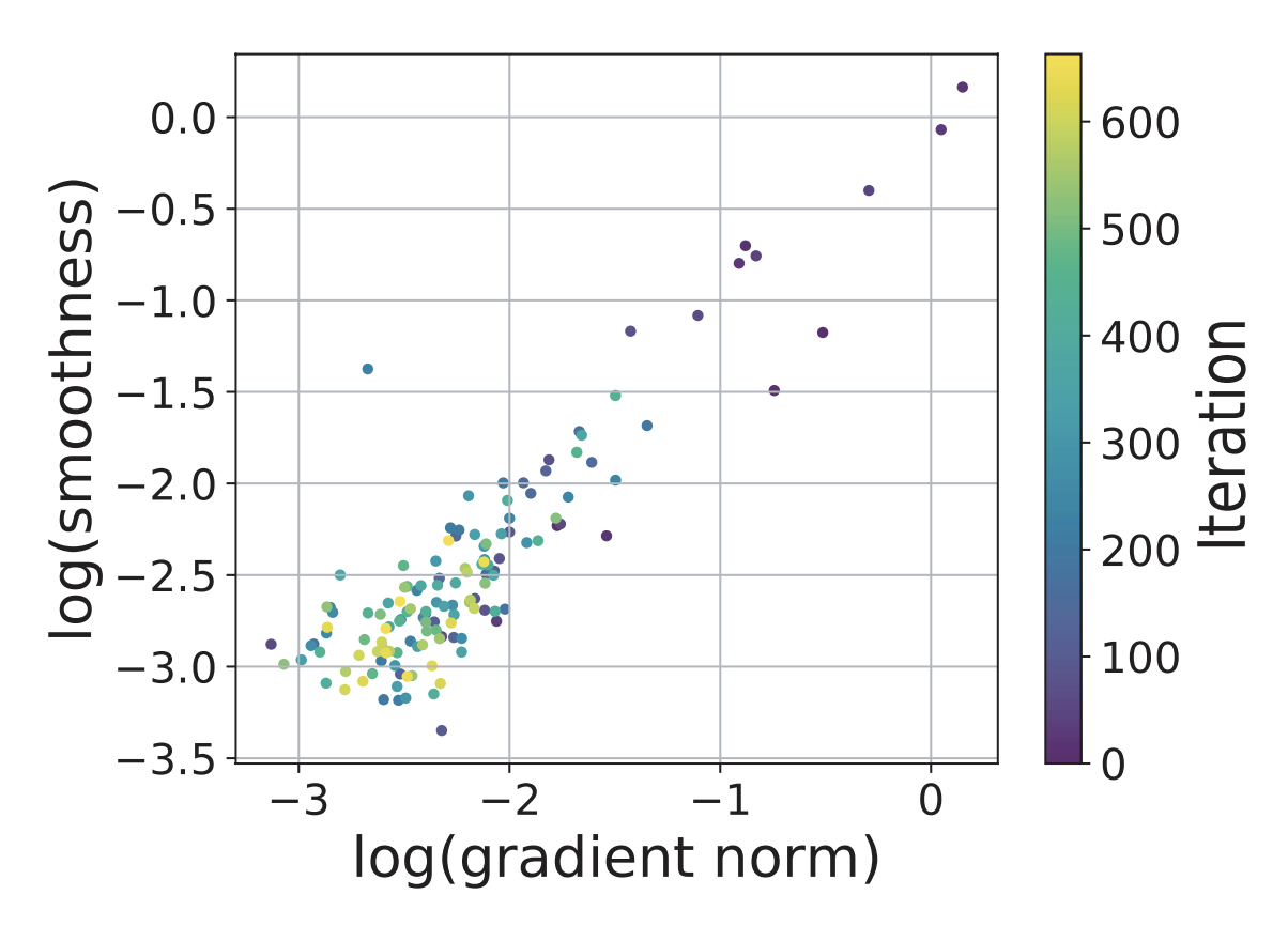
However, I suspect there might be some element of working backward from the desired result; otherwise, who would think to observe the relationship between these two specific quantities?

Under the new constraint, inequality [eq:neq-1] still holds, but with L replaced by the corresponding dynamic term: f(\theta+\Delta\theta) \leq f(\theta) + \left\langle \nabla_{\theta}f(\theta), \Delta\theta\right\rangle + \frac{1}{2}\left(L_0 + L_1\Vert \nabla_{\theta} f(\theta)\Vert\right) \Vert \Delta\theta\Vert^2 Substituting \Delta\theta = -\eta \nabla_{\theta} f(\theta) yields: f(\theta+\Delta\theta) \leq f(\theta) + \left(\frac{1}{2}\left(L_0 + L_1\Vert \nabla_{\theta} f(\theta)\Vert\right)\eta^2 - \eta\right) \Vert \nabla_{\theta}f(\theta)\Vert^2 It is now obvious that to guarantee a decrease at each step, we require: \eta < \frac{2}{L_0 + L_1\Vert \nabla_{\theta} f(\theta)\Vert} And the optimal learning rate is: \eta^* = \frac{1}{L_0 + L_1\Vert \nabla_{\theta} f(\theta)\Vert} This directly leads to gradient clipping as shown in [eq:clip-2]. By ensuring a decrease at every step, it means no effort is wasted during the optimization process, thereby accelerating the training.

Summary

This article briefly introduced a perfect-score ICLR 2020 paper analyzing gradient clipping. The main idea is to introduce more relaxed and universal assumptions. Under these new conditions, the necessity of gradient clipping becomes apparent. Because traditional constraints are relaxed, the theoretical results are more widely applicable, indicating that gradient clipping is indeed a versatile technique suitable for many scenarios.

Original URL: https://kexue.fm/archives/7469

For more details on reposting, please refer to: "Scientific Space FAQ"