Variational Autoencoders (V): VAE + BN = A Better VAE

VAE Training Process

The training process of a VAE can be illustrated as follows:

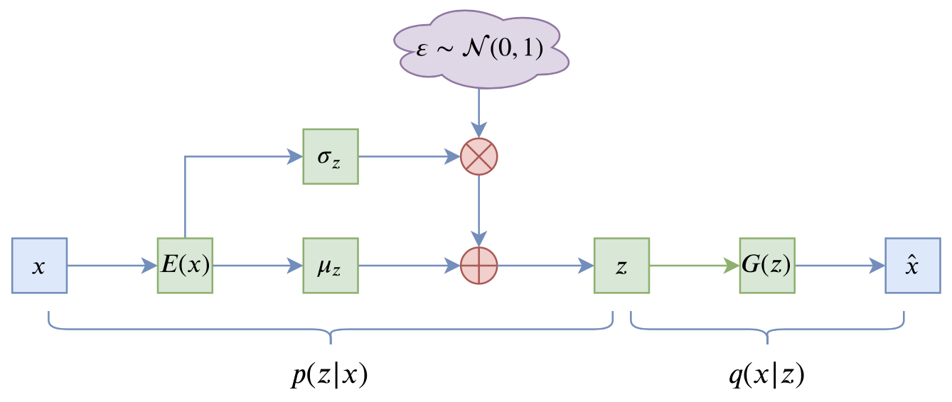
Written as a formula: \mathcal{L} = \mathbb{E}_{x\sim \tilde{p}(x)} \Big[\mathbb{E}_{z\sim p(z|x)}\big[-\log q(x|z)\big]+KL\big(p(z|x)\big\Vert q(z)\big)\Big] The first term is the reconstruction term, where \mathbb{E}_{z\sim p(z|x)} is implemented via reparameterization. The second term is the KL divergence term, which is the explicit difference between a VAE and a standard autoencoder. Without this term, it basically degenerates into a conventional AE. For more detailed symbol definitions, please refer to "Variational Autoencoders (II): From a Bayesian Perspective".

VAE in NLP

In NLP, sentences are encoded as discrete integer IDs, so q(x|z) is a discrete distribution that can be implemented using a powerful "conditional language model." Theoretically, q(x|z) can fit the generative distribution precisely. The problem arises because q(x|z) is too strong. During training, the reparameterization operation introduces noise. When the noise is high, utilizing z becomes difficult. Consequently, the model simply ignores z and degenerates into an unconditional language model (which is still very strong), while KL(p(z|x)\Vert q(z)) drops to 0. This is the KL Vanishing phenomenon.

In this case, the VAE model has little value: a KL divergence of 0 means the encoder outputs a constant vector, and the decoder is just an ordinary language model. Since we use VAEs primarily for their ability to construct encoding vectors unsupervised, we must solve the KL vanishing problem to apply VAEs effectively. In fact, since 2016, many works have addressed this issue, proposing various solutions such as annealing strategies and changing prior distributions. Readers can find many references by searching for "KL Vanishing" on Google.

Brief Derivation

Why is this related to BN? Let’s look at the form of the KL divergence term: \mathbb{E}_{x\sim\tilde{p}(x)}\left[KL\big(p(z|x)\big\Vert q(z)\big)\right] = \frac{1}{b} \sum_{i=1}^b \sum_{j=1}^d \frac{1}{2}\Big(\mu_{i,j}^2 + \sigma_{i,j}^2 - \log \sigma_{i,j}^2 - 1\Big) The above equation is the result of calculating over a sample of b instances, where the encoding vector has d dimensions. Since we always have e^x \geq x + 1, it follows that \sigma_{i,j}^2 - \log \sigma_{i,j}^2 - 1 \geq 0. Therefore: \mathbb{E}_{x\sim\tilde{p}(x)}\left[KL\big(p(z|x)\big\Vert q(z)\big)\right] \geq \frac{1}{b} \sum_{i=1}^b \sum_{j=1}^d \frac{1}{2}\mu_{i,j}^2 = \frac{1}{2}\sum_{j=1}^d \left(\frac{1}{b} \sum_{i=1}^b \mu_{i,j}^2\right) \label{eq:kl} Notice the term in the parentheses; it is the second moment of \mu within the batch. If we add a BN layer to \mu, we can roughly ensure that the mean of \mu is \beta and the variance is \gamma^2 (\beta, \gamma are trainable parameters in BN). At this point: \mathbb{E}_{x\sim\tilde{p}(x)}\left[KL\big(p(z|x)\big\Vert q(z)\big)\right] \geq \frac{d}{2}\left(\beta^2 + \gamma^2\right) \label{eq:kl-lb} So, by controlling \beta and \gamma (mainly by fixing \gamma to a certain constant), we can ensure the KL divergence term has a positive lower bound, thus preventing KL vanishing. In this way, the KL vanishing phenomenon and BN are cleverly linked, using BN to "eliminate" the possibility of KL vanishing.

Why not LN?

Readers skilled in derivation might think that, following the same logic, if the goal is just to give the KL divergence term a positive lower bound, LN (Layer Normalization) could also work—that is, normalizing along the j dimension in Equation [eq:kl].

So why use BN instead of LN?

The answer to this question lies in the cleverness of BN. Intuitively, KL vanishing occurs because the noise in z \sim p(z|x) is relatively large, and the decoder cannot distinguish the non-noise components in z, so it simply discards it. When BN is added to \mu(x), it effectively increases the distance between the z vectors of different samples. This makes it easier to distinguish between them even if z contains noise. Consequently, the decoder becomes willing to use the information in z, alleviating the problem. In contrast, LN performs normalization within a single sample and does not have the effect of pulling apart the distances between different samples, so LN is not as effective as BN.

Connection to the Prior Distribution

For a VAE, we hope that after training, the latent variable distribution of the model matches the prior distribution q(z) = \mathcal{N}(z; 0, 1), while the posterior distribution is p(z|x) = \mathcal{N}(z; \mu(x), \sigma^2(x)). Therefore, the VAE aims for the following to hold: q(z) = \int \tilde{p}(x)p(z|x)dx = \int \tilde{p}(x)\mathcal{N}(z; \mu(x), \sigma^2(x))dx Multiplying both sides by z and integrating over z, we get: 0 = \int \tilde{p}(x)\mu(x)dx = \mathbb{E}_{x\sim \tilde{p}(x)}[\mu(x)] Multiplying both sides by z^2 and integrating over z, we get: 1 = \int \tilde{p}(x)\left[\mu^2(x) + \sigma^2(x)\right]dx = \mathbb{E}_{x\sim \tilde{p}(x)}\left[\mu^2(x)\right] + \mathbb{E}_{x\sim \tilde{p}(x)}\left[\sigma^2(x)\right] If we add BN to both \mu(x) and \sigma(x), we have: \begin{aligned} &0 = \mathbb{E}_{x\sim \tilde{p}(x)}[\mu(x)] = \beta_{\mu}\\ &1 = \mathbb{E}_{x\sim \tilde{p}(x)}\left[\mu^2(x)\right] + \mathbb{E}_{x\sim \tilde{p}(x)}\left[\sigma^2(x)\right] = \beta_{\mu}^2 + \gamma_{\mu}^2 + \beta_{\sigma}^2 + \gamma_{\sigma}^2 \end{aligned} So we now know that \beta_{\mu} must be 0. If we also fix \beta_{\sigma}=0, we obtain the constraint: 1 = \gamma_{\mu}^2 + \gamma_{\sigma}^2 \label{eq:gamma2}

Reference Implementation

Through this derivation, we find that we can add BN to both \mu(x) and \sigma(x), and fix \beta_{\mu}=\beta_{\sigma}=0, while satisfying the constraint in Equation [eq:gamma2]. It should be noted that this part of the discussion is just a general analysis of VAEs and does not yet involve the KL vanishing problem. Even if these conditions are met, there is no guarantee that the KL term won’t tend toward 0. Combining this with Equation [eq:kl-lb], we know that the key to preventing KL vanishing is ensuring \gamma_{\mu} > 0. Therefore, the final strategy I propose is: \begin{aligned} &\beta_{\mu}=\beta_{\sigma}=0\\ &\gamma_{\mu} = \sqrt{\tau + (1-\tau)\cdot\text{sigmoid}(\theta)}\\ &\gamma_{\sigma} = \sqrt{(1-\tau)\cdot\text{sigmoid}(-\theta)} \end{aligned} Where \tau \in (0,1) is a constant (I used \tau=0.5 in my experiments), and \theta is a trainable parameter. The above formula utilizes the identity \text{sigmoid}(-\theta) = 1 - \text{sigmoid}(\theta).

Reference code (Keras):

class Scaler(Layer):
    """Special scale layer
    """
    def __init__(self, tau=0.5, **kwargs):
        super(Scaler, self).__init__(**kwargs)
        self.tau = tau

    def build(self, input_shape):
        super(Scaler, self).build(input_shape)
        self.scale = self.add_weight(
            name='scale', shape=(input_shape[-1],), initializer='zeros'
        )

    def call(self, inputs, mode='positive'):
        if mode == 'positive':
            scale = self.tau + (1 - self.tau) * K.sigmoid(self.scale)
        else:
            scale = (1 - self.tau) * K.sigmoid(-self.scale)
        return inputs * K.sqrt(scale)

    def get_config(self):
        config = {'tau': self.tau}
        base_config = super(Scaler, self).get_config()
        return dict(list(base_config.items()) + list(config.items()))


def sampling(inputs):
    """Reparameterization sampling
    """
    z_mean, z_std = inputs
    noise = K.random_normal(shape=K.shape(z_mean))
    return z_mean + z_std * noise


# Assume e_outputs is the output vector of the encoder
e_outputs  
scaler = Scaler()
z_mean = Dense(hidden_dims)(e_outputs)
z_mean = BatchNormalization(scale=False, center=False, epsilon=1e-8)(z_mean)
z_mean = scaler(z_mean, mode='positive')
z_std = Dense(hidden_dims)(e_outputs)
z_std = BatchNormalization(scale=False, center=False, epsilon=1e-8)(z_std)
z_std = scaler(z_std, mode='negative')
z = Lambda(sampling, name='Sampling')([z_mean, z_std])