Currently, when speaking of "adversarial" in deep learning, it generally carries two meanings: one is Generative Adversarial Networks (GAN), representing a major class of advanced generative models; the other is the field related to adversarial attacks and adversarial examples. While related to GANs, the latter is quite different, primarily concerning the robustness of models under small perturbations. Previous adversarial topics on this blog have focused on the former; today, we will discuss "adversarial training" in the context of the latter.
This article includes the following content:
1. Introduction to basic concepts such as adversarial examples and adversarial training;
2. Introduction to adversarial training based on fast gradient ascent and its application in NLP;
3. Keras implementation of adversarial training (callable with a single line of code);
4. Discussion on the equivalence between adversarial training and gradient penalty;
5. An intuitive geometric understanding of adversarial training based on gradient penalty.
Method Introduction
In recent years, with the rapid development and deployment of deep learning, adversarial examples have received increasing attention. In the field of Computer Vision (CV), we need to enhance model robustness through adversarial attacks and defenses—for example, in autonomous driving systems, preventing a model from misidentifying a red light as green due to random noise. In Natural Language Processing (NLP), similar adversarial training exists, but it is more often used as a regularization technique to improve the model’s generalization ability!
This has made adversarial training one of the "secret weapons" for topping NLP leaderboards. Microsoft surpassed the vanilla RoBERTa on the GLUE leaderboard using RoBERTa combined with adversarial training, and colleagues at my company refreshed the CoQA leaderboard using similar methods. This successfully piqued my interest, leading me to study it and share my findings here.
Basic Concepts
To understand adversarial training, one must first understand "adversarial examples," which first appeared in the paper "Intriguing properties of neural networks." Simply put, they refer to samples that "look" almost identical to humans but result in completely different predictions from the model. A classic example is shown below:
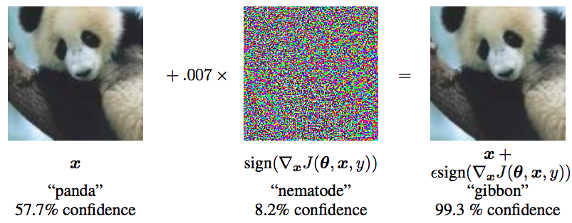
Once adversarial examples are understood, related concepts follow easily. "Adversarial attack" involves finding ways to create more adversarial examples, while "adversarial defense" involves making the model correctly identify them. Adversarial training is a type of defense that incorporates constructed adversarial examples into the original dataset to enhance robustness; as mentioned, in NLP, it also typically improves model performance.
Min-Max
In general, adversarial training can be unified into the following format: \min_{\theta}\mathbb{E}_{(x,y)\sim\mathcal{D}}\left[\max_{\Delta x\in\Omega}L(x+\Delta x, y;\theta)\right] \label{eq:min-max} where \mathcal{D} represents the training set, x is the input, y is the label, \theta represents the model parameters, L(x,y;\theta) is the loss for a single sample, \Delta x is the adversarial perturbation, and \Omega is the perturbation space. This unified format was first proposed in the paper "Towards Deep Learning Models Resistant to Adversarial Attacks."
This formula can be understood in steps:
1. Inject a perturbation \Delta x into x. The goal of \Delta x is to maximize L(x+\Delta x, y;\theta), essentially trying to make the current model’s prediction fail.
2. Of course, \Delta x is not unconstrained; it cannot be too large, or it wouldn’t "look almost identical." Thus, \Delta x must satisfy certain constraints, typically \|\Delta x\| \leq \epsilon, where \epsilon is a constant.
3. After constructing the adversarial example x+\Delta x for each sample, use (x + \Delta x, y) as a data pair to minimize the loss and update parameters \theta (gradient descent).
4. Repeat steps 1, 2, and 3 iteratively.
From this perspective, the entire optimization process is an alternating execution of \max and \min. This is indeed similar to GANs. The difference is that in GANs, the variable for \max is also model parameters, whereas here, the variable for \max is the input (the perturbation amount), meaning a \max step is customized for every single input.
Fast Gradient
The question now is how to calculate \Delta x. Its goal is to increase L(x+\Delta, y;\theta). Since we know that gradient descent decreases loss, the method to increase loss is naturally gradient ascent. Thus, we can simply take: \Delta x = \epsilon \nabla_x L(x, y;\theta) To prevent \Delta x from becoming too large, \nabla_x L(x, y;\theta) is usually standardized. Common methods include: \Delta x = \epsilon \frac{\nabla_x L(x, y;\theta)}{\|\nabla_x L(x, y;\theta)\|} \quad \text{or} \quad \Delta x = \epsilon \operatorname{sign}(\nabla_x L(x, y;\theta)) With \Delta x, we can substitute it back into Equation [eq:min-max] for optimization: \min_{\theta}\mathbb{E}_{(x,y)\sim\mathcal{D}}\left[L(x+\Delta x, y;\theta)\right] This constitutes an adversarial training method known as Fast Gradient Method (FGM), first proposed by the father of GANs, Goodfellow, in the paper "Explaining and Harnessing Adversarial Examples."
Additionally, there is a method called Projected Gradient Descent (PGD), which uses multiple iterations to find a \Delta x that maximizes L(x+\Delta x,y;\theta). However, this article focuses on FGM. For supplementary reading, I recommend the article "Gong Shou Dao: Adversarial Training in NLP + PyTorch Implementation" by Fu Bang.
Back to NLP
For CV tasks, the above process can be executed smoothly. But NLP is different. The input in NLP is text, which is essentially one-hot vectors. Theoretically, "small perturbations" do not exist for one-hot vectors.
A natural idea, as in the paper "Adversarial Training Methods for Semi-Supervised Text Classification," is to add the perturbation to the Embedding layer. While this doesn’t map back to real text, experimental results show that adversarial perturbations at the Embedding layer effectively improve model performance in many tasks.
Experimental Results
Logic Analysis
For NLP tasks, we can directly perturb the Embedding parameter matrix. This serves as a form of regularization and is much easier to implement than deconstructing the model.
Code Reference
Based on the above logic, here is a reference implementation of FGM-based adversarial training for the Embedding layer in Keras:
The core code is as follows:
def adversarial_training(model, embedding_name, epsilon=1):
    """Add adversarial training to the model.
    'model' is the Keras model, and 'embedding_name' is the name
    of the Embedding layer. Use after model.compile().
    """
    if model.train_function is None:
        model._make_train_function()
    old_train_function = model.train_function

    # Find Embedding layer
    for output in model.outputs:
        embedding_layer = search_layer(output, embedding_name)
        if embedding_layer is not None:
            break
    if embedding_layer is None:
        raise Exception('Embedding layer not found')

    # Calculate Embedding gradients
    embeddings = embedding_layer.embeddings
    gradients = K.gradients(model.total_loss, [embeddings])
    gradients = K.zeros_like(embeddings) + gradients[0]

    # Wrap as a function
    inputs = (model._feed_inputs +
              model._feed_targets +
              model._feed_sample_weights)
    embedding_gradients = K.function(
        inputs=inputs,
        outputs=[gradients],
        name='embedding_gradients',
    )

    def train_function(inputs):
        grads = embedding_gradients(inputs)[0]
        delta = epsilon * grads / (np.sqrt((grads**2).sum()) + 1e-8)
        K.set_value(embeddings, K.eval(embeddings) + delta)
        outputs = old_train_function(inputs)
        K.set_value(embeddings, K.eval(embeddings) - delta)
        return outputs

    model.train_function = train_function
Enabling it requires just one line:
adversarial_training(model, 'Embedding-Token', 0.5)Effect Comparison
Tested on CLUE tasks IFLYTEK and TNEWS using BERT base:
| Method | IFLYTEK | TNEWS |
|---|---|---|
| No Adversarial Training | 60.29% | 56.58% |
| With Adversarial Training | 62.46% | 57.66% |
Training script: task_iflytek_adversarial_training.py.
Extended Thinking
In this section, we analyze the results from another perspective, leading to another method of adversarial training and a more intuitive geometric understanding.
Gradient Penalty
Suppose we have the adversarial perturbation \Delta x. When updating \theta, consider the expansion of L(x+\Delta x, y;\theta): \begin{aligned} &\min_{\theta}\mathbb{E}_{(x,y)\sim\mathcal{D}}\left[L(x+\Delta x, y;\theta)\right] \\ \approx&\, \min_{\theta}\mathbb{E}_{(x,y)\sim\mathcal{D}}\left[L(x, y;\theta)+\langle\nabla_x L(x, y;\theta), \Delta x\rangle\right] \end{aligned} The gradient with respect to \theta is: \nabla_{\theta}L(x, y;\theta)+\langle\nabla_{\theta}\nabla_x L(x, y;\theta), \Delta x\rangle Substituting \Delta x=\epsilon \nabla_x L(x, y;\theta), we get: \begin{aligned} &\nabla_{\theta}L(x, y;\theta)+\epsilon\langle\nabla_{\theta}\nabla_x L(x, y;\theta), \nabla_x L(x, y;\theta)\rangle \\ =&\, \nabla_{\theta}\left(L(x, y;\theta)+\frac{1}{2}\epsilon\left\Vert\nabla_x L(x, y;\theta)\right\Vert^2\right) \end{aligned} This suggests that applying a perturbation \epsilon \nabla_x L(x, y;\theta) is approximately equivalent to adding a gradient penalty to the loss: \frac{1}{2}\epsilon\left\Vert\nabla_x L(x, y;\theta)\right\Vert^2 \label{eq:gp}
Geometric Image
We have a very intuitive geometric image for gradient penalty. In a classification problem, the model "digs holes" for each category and places samples of the same category into the same hole:
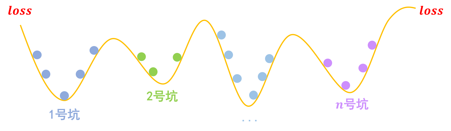
Gradient penalty says: Samples should not only be in the same hole but at the bottom of the hole.
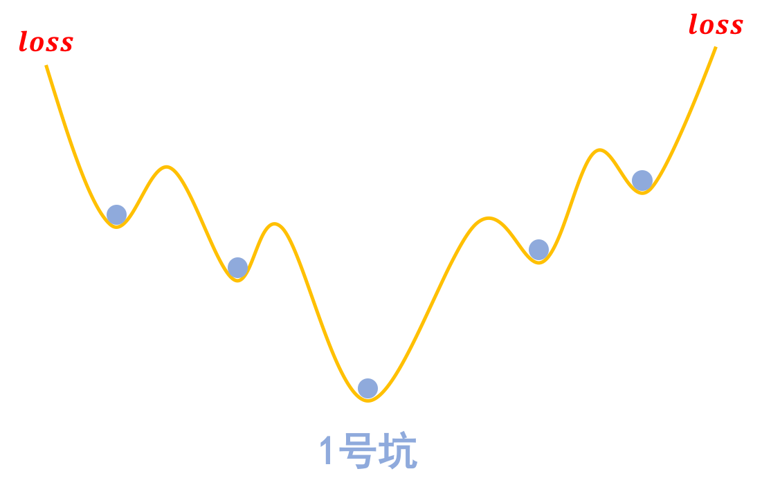
The bottom is the most stable point, making it harder for perturbations to push the sample out of the hole (which would mean a misclassification).
[Click to view GIF: Stability at the bottom of the hole]
![[Click to view GIF: Stability at the bottom of the hole]](https://kexue.fm/usr/uploads/2020/03/3963498733.gif)
The bottom implies a local minimum where the gradient is zero, hence the goal of minimizing \|\nabla_x L(x,y;\theta)\|.
L-Constraint
From the perspective of Lipschitz continuity, a good model should ensure "small input changes lead to small output changes." One way to achieve this is through Spectral Normalization, but it can be overly restrictive. Gradient penalty serves as a softer way to encourage the model to satisfy the L-constraint.
Code Implementation
Gradient penalty is easy to implement as it’s just an extra term in the loss.
def sparse_categorical_crossentropy(y_true, y_pred):
    y_true = K.reshape(y_true, K.shape(y_pred)[:-1])
    y_true = K.cast(y_true, 'int32')
    y_true = K.one_hot(y_true, K.shape(y_pred)[-1])
    return K.categorical_crossentropy(y_true, y_pred)

def loss_with_gradient_penalty(y_true, y_pred, epsilon=1):
    loss = K.mean(sparse_categorical_crossentropy(y_true, y_pred))
    embeddings = search_layer(y_pred, 'Embedding-Token').embeddings
    gp = K.sum(K.gradients(loss, [embeddings])[0].values**2)
    return loss + 0.5 * epsilon * gp

model.compile(
    loss=loss_with_gradient_penalty,
    optimizer=Adam(2e-5),
    metrics=['sparse_categorical_accuracy'],
)
Effect Comparison
Gradient penalty achieves results similar to FGM:
| Method | IFLYTEK | TNEWS |
|---|---|---|
| No Adversarial Training | 60.29% | 56.58% |
| With Adversarial Training (FGM) | 62.46% | 57.66% |
| With Gradient Penalty | 62.31% | 57.81% |
Full code: task_iflytek_gradient_penalty.py.
Summary
This article introduced the basic concepts of adversarial training, focused on the FGM method with Keras implementation, and discussed the connection between adversarial training and gradient penalty with a geometric interpretation.
Original Address: https://kexue.fm/archives/7234