Conditional Random Field (CRF) is a classic method for sequence labeling. It is theoretically elegant and practically effective. Readers who are not yet familiar with CRF are welcome to read my previous post "A Brief Introduction to Conditional Random Fields (CRF) with a Pure Keras Implementation". Since the emergence of the BERT model, many works have explored using BERT+CRF for sequence labeling tasks. However, many experimental results (such as those in the paper "BERT Meets Chinese Word Segmentation") show that for both Chinese word segmentation and named entity recognition tasks, BERT+CRF does not seem to bring much improvement compared to simple BERT+Softmax. This behavior differs from traditional BiLSTM+CRF or CNN+CRF models.
Recently, I added an example of using CRF for Chinese word
segmentation to bert4keras (task_sequence_labeling_cws_crf.py).
During the debugging process, I discovered that the CRF layer might
suffer from insufficient learning. I conducted several comparative
experiments, and the results suggest that this might be the main reason
why CRF provides little improvement in BERT. I am recording the analysis
process here to share with everyone.
The Terrible Transition Matrix
Since I used my own implementation of the CRF layer, to prove that my implementation was correct, I first observed the transition matrix after running the BERT+CRF experiment (using the BERT-base version). The approximate values were as follows:
\begin{array}{c|cccc} & s & b & m & e \\ \hline s & -0.0517 & -0.459 & -0.244 & 0.707 \\ b & -0.564 & -0.142 & 0.314 & 0.613 \\ m & 0.196 & -0.334 & -0.794 & 0.672 \\ e & 0.769 & 0.841 & -0.683 & 0.572 \\ \end{array}
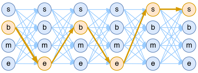
The value in the i-th row and j-th column represents the score of transitioning from i to j (denoted as S_{i\to j}). The absolute values of the scores are meaningless; only their relative values matter. As a side note, the Chinese word segmentation in this article uses the (s, b, m, e) character tagging method. If you are unfamiliar with this, you can refer to "Chinese Word Segmentation Series: 3. Character Tagging and HMM Models".
Intuitively, however, this does not look like a well-learned transition matrix; it might even have a negative impact. For example, looking at the first row, S_{s\to b} = -0.459 and S_{s\to e} = 0.707. That is, S_{s\to b} is significantly smaller than S_{s\to e}. However, according to the (s, b, m, e) tagging design, it is possible for s to be followed by b, but impossible for it to be followed by e. Therefore, S_{s\to b} < S_{s\to e} is clearly unreasonable. it could lead to invalid tag sequences. Ideally, S_{s\to e} should be -\infty.
This unreasonable transition matrix once made me think there was a problem with my CRF implementation. But after repeated checks and comparisons with the official Keras implementation, I finally confirmed that my implementation was correct. So where is the problem?
Learning Rate Imbalance
If we ignore the rationality of this transition matrix for a moment and directly apply the Viterbi algorithm for decoding and prediction based on the training results, and then evaluate it with the official script, we find that the F1 score is around 96.1% (on the PKU task), which is already at the state-of-the-art level.
The transition matrix is terrible, yet the final result is still very good. This only indicates that the transition matrix has almost no impact on the final result. Under what circumstances does the transition matrix have almost no impact? A possible reason is that the tag scores for each character output by the model are much larger than the values in the transition matrix, and the discriminative power is already very clear. Consequently, the transition matrix cannot influence the overall result. In other words, at this point, simply using Softmax and taking the argmax is already sufficient. To confirm this, I randomly selected some sentences and observed the tag distribution for each character. I indeed found that the highest tag score for each character was generally between 6 and 8, while the other tag scores were generally more than 3 points lower than the highest one. This is more than an order of magnitude larger than the values in the transition matrix, making it difficult for the transition matrix to exert any influence. This confirms the hypothesis.
A good transition matrix should obviously help with prediction, at least by helping us exclude unreasonable tag transitions, or at least ensuring it doesn’t bring negative effects. So it is worth considering: What exactly prevents the model from learning a good transition matrix? I suspect the answer is the learning rate.
When fine-tuning BERT for downstream tasks after pre-training, only a very small learning rate is needed (usually on the order of 10^{-5}); if it’s too large, the model might not converge. Although the learning rate is small, convergence is fast for most downstream tasks, with many tasks requiring only 2 to 3 epochs to reach the optimum. On the other hand, BERT has a very strong fitting capability, so it can fit the training data quite thoroughly.
What does this imply? First, we know that the tag distribution for each character is calculated directly by the BERT model, while the transition matrix is an addition that is not directly related to BERT. When we fine-tune with a learning rate of 10^{-5}, the BERT part converges rapidly, meaning the tag distribution for each character is fitted quickly. Because BERT’s fitting capability is strong, it quickly reaches a relatively optimal state (where the target tag score is high and the gap with non-target tags is wide). Since the transition matrix has little connection to BERT, while the character-wise tag distribution converges rapidly to an optimal value, the transition matrix still moves "leisurely" at a speed of 10^{-5}, eventually ending up an order of magnitude lower than the character-wise scores. Furthermore, once the character-wise tag distributions can already fit the target sequence well, the transition matrix is no longer needed (the gradient of the transition matrix will be very small, resulting in almost no updates).
Thinking about this, a natural idea is: Can we increase the learning rate of the CRF layer? I tried increasing the learning rate of the CRF layer. After several experiments, I found that when the learning rate of the CRF layer is more than 100 times the main learning rate, the transition matrix begins to become reasonable. Below is a transition matrix trained when the BERT main learning rate was 10^{-5} and the CRF layer learning rate was 10^{-2} (i.e., 1000 times larger):
\begin{array}{c|cccc} & s & b & m & e \\ \hline s & 3.17 & 2.16 & -3.97 & -2.04 \\ b & -3.89 & -0.451 & 1.67 & 0.874 \\ m & -3.9 & -4.41 & 3.82 & 2.45 \\ e & 1.88 & 0.991 & -2.48 & -0.247 \\ \end{array}
Such a transition matrix is reasonable, and the magnitude is correct. It has learned the correct tag transitions, such as s\to s, b having higher scores than s\to m, e, and b\to m, e having higher scores than b\to s, b, and so on. However, even if the learning rate of the CRF layer is increased, the results do not show a significant advantage compared to when it is not adjusted. Ultimately, BERT’s fitting capability is too strong; even the Softmax effect can reach the optimum, so the transition matrix naturally cannot bring much improvement.
(Note: For techniques on increasing the learning rate, you can refer to "Make Keras Cooler: Layer-wise Learning Rates and Free Gradients".)
More Experimental Analysis
The reason CRF didn’t bring much change to BERT is that BERT’s fitting capability is too strong, making the results very good even without a transition matrix. So, if we reduce BERT’s fitting capability, will it lead to significant differences?
In the previous experiments, the output of the 12th layer of BERT-base was used for fine-tuning. Now, we use only the output of the 1st layer for fine-tuning to test whether the above adjustments bring significant differences. The results are shown in the table below:
| Main LR | CRF LR | Epoch 1 Test F1 | Best Test F1 | |
|---|---|---|---|---|
| CRF-1 | 10^{-3} | 10^{-3} | 0.914 | 0.925 |
| CRF-2 | 10^{-3} | 10^{-2} | 0.929 | 0.930 |
| CRF-3 | 10^{-2} | 10^{-2} | 0.673 | 0.747 |
| Softmax | 10^{-3} | - | 0.899 | 0.907 |
Since only one layer of BERT was used, the main learning rate was set to 10^{-3} (the shallower the model, the larger the learning rate can appropriately be). The main comparison is the improvement brought by adjusting the CRF layer’s learning rate. From the table, we can see:
1. Under an appropriate learning rate, CRF performs better than Softmax;
2. Appropriately increasing the learning rate of the CRF layer also provides a certain improvement over the original CRF.
This indicates that for models whose fitting capability is not particularly strong (such as using only the first few layers of BERT, or for certain particularly difficult tasks where even the full BERT’s fitting capability is not sufficient), CRF and its transition matrix are still helpful, and fine-tuning the learning rate of the CRF layer can bring even greater improvements. Furthermore, all the above experiments were conducted based on BERT. Does the same approach work for traditional BiLSTM+CRF or CNN+CRF? I also did a simple experiment and found that it is helpful in some cases, so I estimate this is a general trick for CRF layers.
Summary
Starting from the CRF example added to bert4keras, this
article discovered that when BERT is combined with CRF, the CRF layer
may suffer from insufficient training. It then hypothesized the possible
reasons and further confirmed the hypothesis through experiments.
Finally, it proposed increasing the learning rate of the CRF layer to
improve the effect of CRF and preliminarily verified its effectiveness
(under certain tasks).
When reprinting, please include the original address of this article: https://kexue.fm/archives/7196
For more detailed reprinting matters, please refer to: "Scientific Space FAQ"