From Denoising Autoencoders to Generative Models

Denoising Autoencoders

The fundamental starting point for both papers is the Denoising Autoencoder; more precisely, they utilize the optimal solution of a Denoising Autoencoder.

Basic Result: If x, \varepsilon \in \mathbb{R}^d, with x \sim p(x) and \varepsilon \sim u(\varepsilon), where u(\varepsilon) = \mathcal{N}(0, \sigma^2 I_d), then: \begin{aligned} r(x) &= \mathop{\text{argmin}}_{r} \mathbb{E}_{x \sim p(x), \varepsilon \sim \mathcal{N}(0, \sigma^2 I_d)} \left[ \| r(x + \varepsilon) - x \|^2 \right] \\ &= x + \sigma^2 \nabla_x \log \hat{p}(x) \end{aligned} \label{eq:denoise}

Here, \hat{p}(x) = [p * u](x) = \int p(x-\varepsilon)u(\varepsilon) d\varepsilon = \int p(\varepsilon)u(x-\varepsilon) d\varepsilon refers to the convolution of the distributions p(x) and u(\varepsilon). Specifically, it represents the probability density of x + \varepsilon. In other words, if p(x) represents the distribution of real images, then sampling from \hat{p}(x) yields a set of real images with added Gaussian noise.

The result in Eq. [eq:denoise] means that the optimal denoising autoencoder for additive Gaussian noise can be calculated explicitly, and the result is related to the gradient of the distribution. This result is very interesting and profound, worth reflecting upon. For instance, Eq. [eq:denoise] tells us that r(x) - x is actually an estimate of the gradient of the (noisy) real distribution. Having the gradient of the real distribution allows us to do many things, especially regarding generative models.

Proof: The proof of Eq. [eq:denoise] is not difficult. Taking the variation of the objective: \begin{aligned} & \delta \iint p(x)u(\varepsilon) \| r(x + \varepsilon) - x \|_2^2 dx d\varepsilon \\ =& \delta \iint p(x)u(y-x) \| r(y) - x \|_2^2 dx dy \\ =& 2 \iint p(x)u(y-x) \langle r(y) - x, \delta r(y) \rangle dx dy \end{aligned} Setting this to zero, we get \int p(x)u(y-x)(r(y) - x)dx = 0, which implies: r(y) = \frac{\int p(x)u(y-x)x dx}{\int p(x)u(y-x) dx} Substituting the expression u(\varepsilon) = \frac{1}{(2\pi \sigma^2)^{d/2}} \exp\left( -\frac{\| \varepsilon \|_2^2}{2\sigma^2} \right), we obtain: r(y) = y + \sigma^2 \nabla_y \log [p * u](y)

A Winding Path

We first introduce the approach of "Learning Generative Models using Denoising Density Estimators". Following the usual conventions of GANs and VAEs, we hope to train a mapping x = G(z) such that z sampled from a prior distribution q(z) is mapped to a real sample. In probabilistic terms, we want to minimize the distance between p(x) and the following q(x): q(x) = \int q(z) \delta(x - G_{\theta}(z)) dz To this end, a common optimization objective for GANs is to minimize KL(q(x) \| p(x)). However, since we have an estimate for the gradient of \hat{p}(x), we can change the objective to minimizing KL(\hat{q}(x) \| \hat{p}(x)).

We can perform the following derivation: \begin{aligned} KL(\hat{q}(x) \| \hat{p}(x)) &= \int \hat{q}(x) \log \frac{\hat{q}(x)}{\hat{p}(x)} dx \\ &= \int q(x)u(\varepsilon) \log \frac{\hat{q}(x+\varepsilon)}{\hat{p}(x+\varepsilon)} dx d\varepsilon \\ &= \int q(z)\delta(x-G_{\theta}(z))u(\varepsilon) \log \frac{\hat{q}(x+\varepsilon)}{\hat{p}(x+\varepsilon)} dx d\varepsilon dz \\ &= \int q(z)u(\varepsilon) \log \frac{\hat{q}(G_{\theta}(z)+\varepsilon)}{\hat{p}(G_{\theta}(z)+\varepsilon)} d\varepsilon dz \\ &= \mathbb{E}_{z \sim q(z), \varepsilon \sim u(\varepsilon)} \left[ \log \hat{q}(G_{\theta}(z)+\varepsilon) - \log \hat{p}(G_{\theta}(z)+\varepsilon) \right] \end{aligned} \label{eq:dae-1} This objective requires estimates of \log \hat{p}(x) and \log \hat{q}(x). We can construct two \mathbb{R}^d \to \mathbb{R} models E_p(x) and E_q(x) using neural networks, and minimize: \begin{aligned} \mathop{\text{argmin}}_{E_p} \mathbb{E}_{x \sim p(x), \varepsilon \sim \mathcal{N}(0, \sigma^2 I_d)} \left[ \| \nabla_x E_p(x + \varepsilon) + \varepsilon \|^2 \right] \\ \mathop{\text{argmin}}_{E_q} \mathbb{E}_{x \sim q(x), \varepsilon \sim \mathcal{N}(0, \sigma^2 I_d)} \left[ \| \nabla_x E_q(x + \varepsilon) + \varepsilon \|^2 \right] \end{aligned} \label{eq:e-grad} That is, we use \nabla_x E_p(x) + x and \nabla_x E_q(x) + x as denoising autoencoders. According to Eq. [eq:denoise], we have: \left\{ \begin{aligned} \nabla_x E_p(x) + x &= x + \sigma^2 \nabla_x \log \hat{p}(x) \\ \nabla_x E_q(x) + x &= x + \sigma^2 \nabla_x \log \hat{q}(x) \end{aligned} \right. \quad \Rightarrow \quad \left\{ \begin{aligned} E_p(x) &= \sigma^2 \log \hat{p}(x) + C_1 \\ E_q(x) &= \sigma^2 \log \hat{q}(x) + C_2 \end{aligned} \right. In other words, up to a constant, E_p(x) is proportional to \log \hat{p}(x) and E_q(x) is proportional to \log \hat{q}(x). Since constants do not affect optimization, we can substitute E_p(x) and E_q(x) into Eq. [eq:dae-1] to get: KL(\hat{q}(x) \| \hat{p}(x)) \sim \mathbb{E}_{z \sim q(z), \varepsilon \sim u(\varepsilon)} \left[ E_q(G_{\theta}(z)+\varepsilon) - E_p(G_{\theta}(z)+\varepsilon) \right] \label{eq:dae-2}

This yields a workflow for a generative model:

Select a prior distribution q(z), initialize G_{\theta}(z), and pre-calculate E_p(x). Loop through the following 3 steps until convergence:

1. Sample a batch z \sim q(z) and a batch of noise \varepsilon \sim \mathcal{N}(0, \sigma^2 I_d), and synthesize a batch of noisy fake samples x = G_{\theta}(z) + \varepsilon;

2. Use this batch of noisy fake samples to train E_q(x);

3. Fix E_p and E_q, and update G_{\theta} for several steps using gradient descent based on Eq. [eq:dae-2].

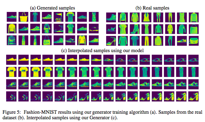
The experiments in this paper are relatively simple, only covering MNIST and Fashion MNIST, but they demonstrate its feasibility:

A Sudden Turn

The other paper, "Annealed Denoising Score Matching: Learning Energy-Based Models in High-Dimensional Spaces", is even more direct. It is essentially a combination of Denoising Autoencoders and Energy-Based Models.

Since Eq. [eq:denoise] has already helped us obtain \nabla_x \log \hat{p}(x) = (r(x) - x) / \sigma^2 (of course, the actual implementation in this paper does not directly use a neural network to fit r(x), but rather fits a scalar function like in Eq. [eq:e-grad], but the idea remains the same), this allows us to sample from \hat{p}(x). Of course, the sampled images will have noise, so we need to pass the sampling results through r(x) to denoise them: p(x) = \mathbb{E}_{x_{noise} \sim \hat{p}(x)} [ \delta(x - r(x_{noise})) ]

So, how specifically do we sample from \hat{p}(x)? Langevin dynamics! Since we know \nabla_x \log \hat{p}(x), the following Langevin equation: x_{t+1} = x_t + \frac{1}{2}\varepsilon \nabla_x \log \hat{p}(x) + \sqrt{\varepsilon}\alpha, \quad \alpha \sim \mathcal{N}(0, 1) \label{eq:sde} will have \hat{p}(x) as its stationary distribution as \varepsilon \to 0 and t \to \infty. In other words, the sequence \{x_t\} will follow the distribution \hat{p}(x).

Thus, the process of sampling from \hat{p}(x) is solved by this direct (though perhaps less elegant) method. After training the Denoising Autoencoder, a generative model is automatically obtained.

The overall process is:

1. Train a denoising autoencoder r(x) to obtain \nabla_x \log \hat{p}(x);

2. Use the iterative process in Eq. [eq:sde] to sample, resulting in a batch of noisy real samples;

3. Pass the sampling results from step 2 through r(x) to denoise them, obtaining noise-free samples.

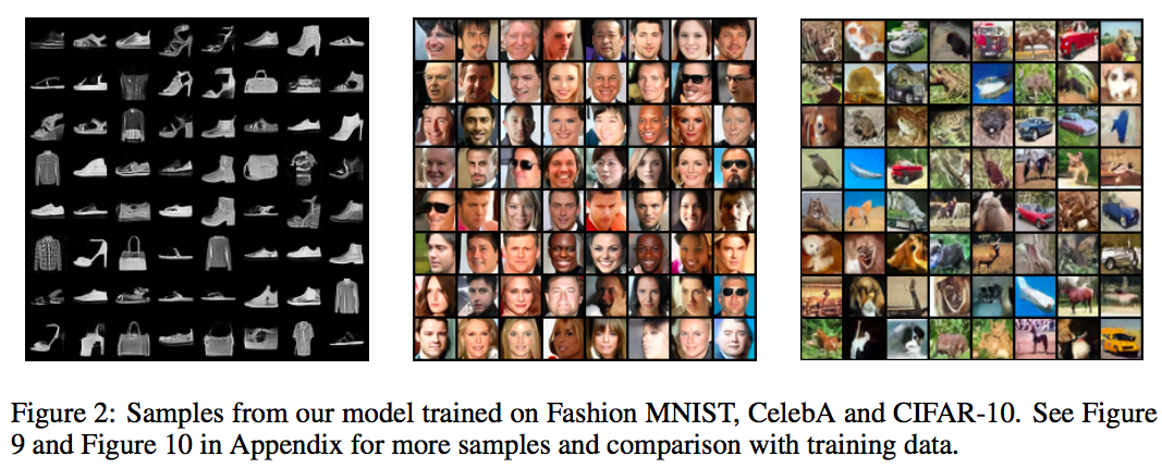
Of course, the paper contains many more details. The core technique is the use of an annealing strategy to stabilize the training process and improve generation quality. I am not particularly interested in those details, as I mainly want to learn novel ideas for generative models to broaden my horizons. However, it must be said that despite the directness of the approach, the generation results are quite competitive, showing impressive performance on Fashion MNIST, CelebA, and CIFAR-10:

Conclusion

This article introduced two similar papers submitted to ICLR 2020, both utilizing Denoising Autoencoders to build generative models. Since I had not encountered these specific ideas before, I read them with great interest.

Regardless of the generation quality, I find them quite inspiring and they have sparked some thoughts (not only in CV but also in NLP). For example, BERT’s MLM pre-training method is essentially a denoising autoencoder. Is there a result similar to Eq. [eq:denoise] for it? Conversely, can results like Eq. [eq:denoise] inspire us to construct new pre-training tasks, or help clarify the underlying principles of the pretrain + finetune workflow?

When reposting, please include the original address of this article: https://kexue.fm/archives/7038

For more details on reposting, please refer to: "Scientific Space FAQ"