Let us tirelessly review: the Minimum Entropy Principle is a principle for unsupervised learning. "Entropy" represents the learning cost, and reducing this cost is our relentless pursuit. By "minimizing the learning cost," we can learn many results in an unsupervised manner that align with our cognitive understanding. This is the basic philosophy of the Minimum Entropy Principle.
In this article, we will introduce a quite beautiful clustering algorithm that also embodies the Minimum Entropy Principle—or rather, it can be derived from it. It is called InfoMap, or MapEquation. In fact, InfoMap is a result from 2007, with the earliest paper being "Maps of random walks on complex networks reveal community structure." Although it may seem old, I believe it remains the most beautiful clustering algorithm currently available. This is because it not only tells us how to cluster but, more importantly, provides an elegant information-theoretic explanation for why we cluster, and directly derives the entire clustering process from this explanation.
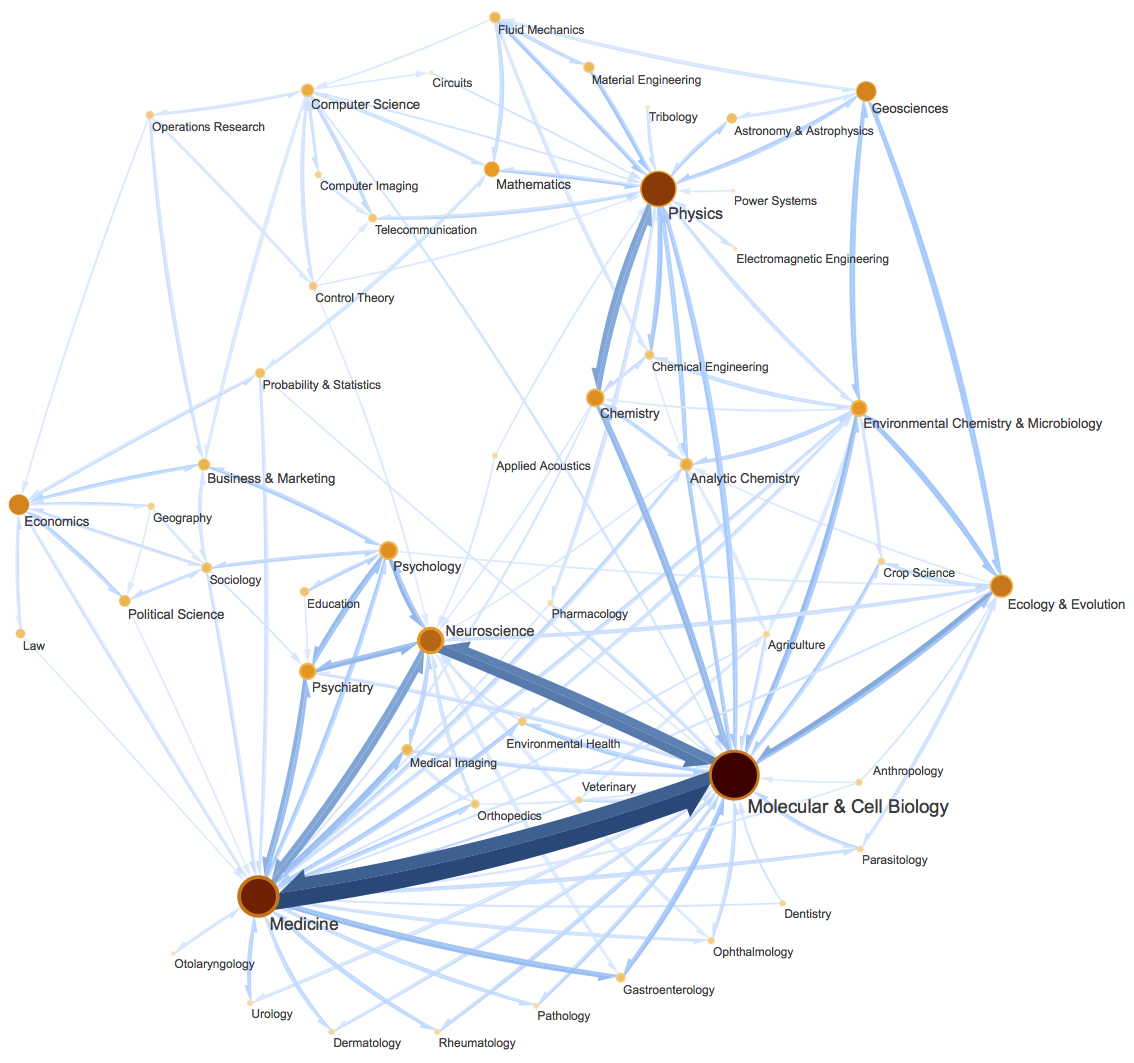
Of course, its scope is not limited to clustering; more accurately, it is a "community detection" algorithm on graph networks. Community Detection roughly means given a directed or undirected graph network, finding the "clumping" or "grouping" behavior within the network. For detailed meanings, you can search for it yourself. Simply put, it is similar to clustering but richer in meaning (see also "What is Community Detection?").
Entropy and Coding
In previous articles, we used the concept of information entropy to describe related ideas. Starting from this article, we introduce an equivalent concept of information entropy—average code length. Introducing this helps us more precisely understand and construct the objective of minimum entropy.
Binary Tree Coding
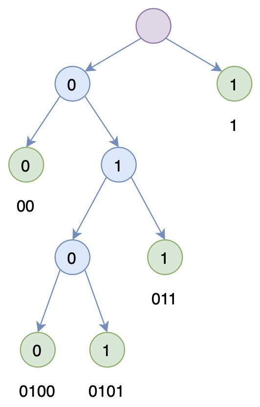
Coding refers to using combinations of a finite set of markers to represent original information. The most typical is binary coding, using only the digits 0 and 1. A code usually has a one-to-one correspondence with the original object. For example, "Science" might correspond to (11, 1001) if "Sci" is 11 and "ence" is 1001.
Note that we are considering static coding here, where each encoded object corresponds one-to-one with a code result. We also consider prefix-free codes (no-separator codes), meaning we can decode individual objects without extra separators. This requires that no code is a prefix of any other code (so we only need to read bits until an object is recognized, then start over). This implies that all codes can be constructed into a binary tree where each code corresponds to a leaf, as shown in the figure.
Based on this, we can reach a very interesting and significant conclusion: assuming n different characters with code lengths l_1, l_2, \dots, l_n, we have: \sum_{i=1}^n 2^{-l_i} \leq 1 \label{eq:leq} This is a direct corollary of the binary tree representation; readers can attempt to prove it themselves.
Shortest Code Length
Imagine a "shorthand" scenario where we need to quickly record spoken words. The recording method involves mapping each word to a binary code. To record faster, we naturally want frequently occurring words to have shorter codes. For example, if the word "the" appears very frequently, using a long string like 11000010001 would slow us down, whereas using a short code like 10 would significantly improve recording speed.
Suppose there are n different characters with occurrence probabilities P = (p_1, p_2, \dots, p_n). We might be interested in two questions: First, how do we find the optimal coding scheme to minimize the total average code length? Second, what is the theoretical minimum for this average code length?
For the first question, the answer is Huffman coding (the same Huffman used in Huffman Softmax in Word2Vec), but that is not the focus here. For the second question, the answer is a fundamental result in information theory: it is exactly the Information Entropy: H(P) = -\sum_{i=1}^n p_i \log_2 p_i \label{eq:l} In other words, information entropy is precisely the theoretical shortest average code length. Note that this is a very "powerful" result; it tells us that no matter what coding you use (with or without separators, static or dynamic), the average code length cannot be lower than \eqref{eq:l}.
Here we provide a simple proof of \eqref{eq:l} for the prefix-free coding scenario. Let the code lengths of n characters be l_1, l_2, \dots, l_n. We calculate the average code length: \sum_{i=1}^n p_i l_i = -\sum_{i=1}^n p_i \log_2 2^{-l_i} \label{eq:avg-l} Because of the inequality \eqref{eq:leq}, we define: \hat{p} = 1 - \sum_{i=1}^n 2^{-l_i} \geq 0 Then equation \eqref{eq:avg-l} can be written as: - 0 \times \log \hat{p} - \sum_{i=1}^n p_i \log_2 2^{-l_i} This is the cross-entropy between the probability distributions P = (0, p_1, p_2, \dots, p_n) and Q = (\hat{p}, 2^{-l_1}, 2^{-l_2}, \dots, 2^{-l_n}). Since cross-entropy is minimized when P=Q (derived from KL(P \Vert Q) \geq 0), we finally have: \sum_{i=1}^n p_i l_i \geq -\sum_{i=1}^n p_i \log_2 p_i
Readers familiar with information theory should know this conclusion. It tells us that the shortest average code length is the entropy, which is also the limit of lossless compression. We seek better schemes to approach this limit, which is the essence of minimum entropy.
Finally, since different logarithmic bases only result in a constant scale factor, we usually do not specify the base, or we default to the natural logarithm for simpler theoretical forms.
InfoMap
Returning to InfoMap, it is directly related to the compression coding mentioned above. In fact, my supervisor introduced InfoMap to me during my first year of graduate school, but unfortunately, I didn’t truly understand its origins until recently. The reason for the delay was partly my lack of familiarity with entropy and coding theory, and partly because the original authors might not have realized where the bottleneck for non-information-theory readers lies.
I decided to write down my understanding, hoping to help more readers grasp InfoMap, as it is truly beautiful.
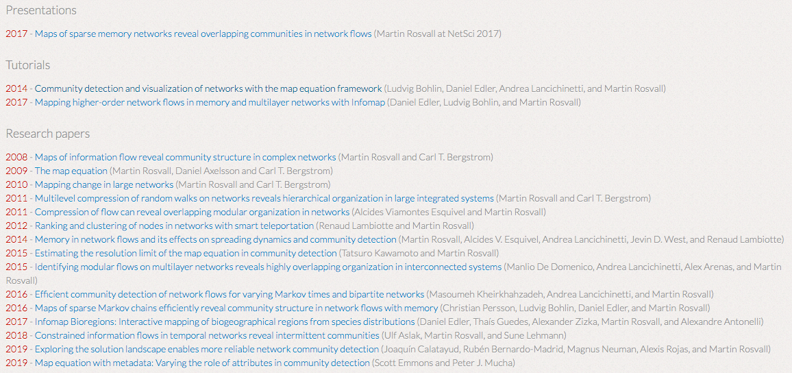
InfoMap Publication List: https://www.mapequation.org/publications.html
(The fact that a website was created specifically for one algorithm, and that it remains active today, shows the authors’ passion and the algorithm’s effectiveness.)
Categorical Memory
Suppose we are tasked with memorizing the following sequence in a short time:

The sequence is not long, and to form a memory quickly, your strategy might be:
The first 3 are fruits; the middle 5 are cities; the last 4 are Arabic numerals.
The 3 fruits are Pear, Grape, Banana.
The 5 cities are Guangzhou, Shanghai, Beijing, Hangzhou, Shenzhen.
The 4 numbers are 123, 654, 798, 963.
In other words, everyone essentially thinks in terms of grouping by category. This makes memory more efficient. The Minimum Entropy Principle tells us that "efficiency" and "effort-saving" are mathematically described by the reduction of entropy. Therefore, a good classification scheme should satisfy the minimum entropy principle, reducing the system’s entropy. This is the core optimization goal of InfoMap: seeking the optimal clustering scheme by minimizing entropy.
Hierarchical Coding: Concept
As mentioned, information entropy is equivalent to the shortest code length, so minimum entropy is essentially looking for better compression algorithms. If grouping memory is more efficient, there must be a coding method that compresses information more effectively. This method is hierarchical coding.
In hierarchical coding, we no longer use a single code to represent an object. Instead, we use a combination of two (or more) codes: the first represents the object’s category, and the second represents its index within that category. If objects of the same category often appear "bunched together," hierarchical coding can compress the data.
How does hierarchical coding compress? Unfortunately, most InfoMap materials do not emphasize the specific encoding process. I believe this process should be highlighted for clarity:

Note that the coding must be lossless; there must be a way to decode it back to the original sequence. To achieve this, hierarchical coding inserts category markers and exit markers into the original sequence. Category markers use one set of codes, while objects within the category and the exit marker use another set. Because categories are distinct, objects in different categories can reuse the same code (e.g., "Pear" and "Shanghai" could both be 001), reducing the overall average code length. When decoding, once a category code is read, the decoder uses that category’s internal codes until an exit marker appears, then it looks for a new category code.
Hierarchical Coding: Calculation
Now that we’ve established that this coding is lossless, we need to calculate it. The conclusion that "average code length is shortened" must be supported by quantitative results.
Assume we have a specific hierarchical coding scheme. We can calculate its average code length. Define the following notations:
| Notation | Meaning |
|---|---|
| p_{\alpha} | Probability of occurrence of object \alpha |
| q_{i\curvearrowright} | Probability of exiting category i |
According to our coding convention, every category sequence must end with that category’s exit marker, so q_{i\curvearrowright} is also the probability of the exit marker for category i. It is important to emphasize that these probabilities are globally normalized, meaning: \underbrace{\sum_i q_{i\curvearrowright}}_{\text{Sum of category entry probabilities}} + \underbrace{\sum_{\alpha} p_{\alpha}}_{\text{Sum of object probabilities}} + \underbrace{\sum_i q_{i\curvearrowright}}_{\text{Sum of exit marker probabilities}} = 1 \label{eq:guiyi} Since categories and internal objects use two different sets of codes, we calculate them separately. The shortest average code length for categories is: H(\mathcal{Q}) = -\sum_i \frac{q_{i\curvearrowright}}{q_{\curvearrowright}} \log \frac{q_{i\curvearrowright}}{q_{\curvearrowright}} where q_{\curvearrowright} = \sum_i q_{i\curvearrowright}. This is because category codes are independent; normalizing their probabilities within the category set and applying the entropy formula gives the theoretical shortest average code length for categories.
Similarly, the shortest average code length for objects within category i is: H(\mathcal{P}^i) = - \frac{q_{i\curvearrowright}}{p_{i\circlearrowright}} \log \frac{q_{i\curvearrowright}}{p_{i\circlearrowright}} - \sum_{\alpha \in i} \frac{p_{\alpha}}{p_{i\circlearrowright}} \log \frac{p_{\alpha}}{p_{i\circlearrowright}} where p_{i\circlearrowright} = q_{i\curvearrowright} + \sum_{\alpha \in i} p_{\alpha}. Note: Distinguish the notations carefully (p vs q? \curvearrowright vs \circlearrowright?). Misinterpreting these will make understanding much harder. The formula means that objects in each category use their own code set, so we normalize the object probabilities and the exit marker probability within that category and apply the entropy formula.
Finally, the weighted average of both gives the total shortest average code length: L(M) = \textcolor{red}{q_{\curvearrowright}H(\mathcal{Q})} + \textcolor{cyan}{\sum_i p_{i\circlearrowright} H(\mathcal{P}^i)} \label{eq:loss}
Now we have a quantitative indicator \eqref{eq:loss} to compare different hierarchical coding schemes. Conversely, given a sequence of objects, we can search for a hierarchical coding scheme that minimizes \eqref{eq:loss}, thereby finding an optimal clustering. Note that this clustering algorithm has almost no hyperparameters—given the sequence, we find the coding that minimizes \eqref{eq:loss} without needing to specify the number of clusters beforehand.
Random Walk
So far, we have an optimization objective \eqref{eq:loss} to cluster objects in a given sequence. But we haven’t linked this to classic clustering tasks yet, which usually provide similarity between samples rather than a sequence.
InfoMap handles this by abstracting the samples into a directed graph. Each sample is a node, and any two nodes (\alpha, \beta) have an edge \beta \to \alpha with a weight representing the transition probability p_{\beta \to \alpha}. For a general graph, edges represent similarity, which can be normalized to represent transition probabilities.
With this setup, the classic idea of a "Random Walk" emerges: start at node j, jump to node i with probability p(i|j), and repeat. This generates a very long sequence. Once we have the sequence, we can use \eqref{eq:loss} as the objective for clustering.
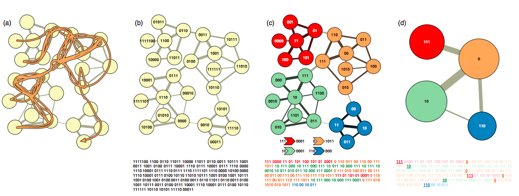
This is the InfoMap clustering process: Construct transition probabilities, perform a random walk on the graph to generate a sequence, apply hierarchical coding to the sequence, and minimize \eqref{eq:loss} to complete the clustering.
Incidentally, when DeepWalk (2014) proposed using random walks on graphs to generate sequences for Word2Vec, many found it revolutionary. However, the idea of using random walks on graphs has clearly been around for a long time.
The Math of InfoMap
Let’s make the process more mathematically rigorous.
First, we don’t actually need to simulate the random walk. We only need the steady-state probabilities of the objects in the sequence. To find these, we solve: \begin{pmatrix} p_1 \\ p_2 \\ \vdots \\ p_n \end{pmatrix} = \begin{pmatrix} p_{1\to 1} & p_{2\to 1} & \cdots & p_{n\to 1} \\ p_{1\to 2} & p_{2\to 2} & \cdots & p_{n\to 2} \\ \vdots & \vdots & \ddots & \vdots \\ p_{1\to n} & p_{2\to n} & \cdots & p_{n\to n} \end{pmatrix} \begin{pmatrix} p_1 \\ p_2 \\ \vdots \\ p_n \end{pmatrix} \label{eq:pab} or p_{\beta} = \sum_{\alpha} p_{\alpha} p_{\alpha \to \beta}. This means if the steady-state distribution is (p_1, \dots, p_n), one more step of the random walk leaves the distribution unchanged.
However, a simple random walk might depend on the initial values—the solution to \eqref{eq:pab} might not be unique. If the graph has isolated regions, the walk might get stuck. To solve this, the authors introduced a "teleportation probability" \tau: with probability 1-\tau, follow the transition probabilities p_{\beta \to \alpha}; with probability \tau, jump to any random node in the graph. The equation becomes: p_{\beta} = (1-\tau)\sum_{\alpha} p_{\alpha} p_{\alpha \to \beta} + \tau \sum_{\alpha} \frac{p_{\alpha}}{n} \label{eq:pa} This effectively changes the transition probability to (1-\tau)p_{\alpha \to \beta} + \tau/n.
With teleportation, the model avoids local traps, ensuring a unique solution. The authors used \tau = 0.15. For more details on robustness, see "The map equation" and "Community detection and visualization of networks with the map equation framework."
Now we have p_{\alpha}. We still need q_{i\curvearrowright}, the exit probability. This is the probability that the random walk leaves category i: q_{i\curvearrowright} = \sum_{\alpha \in i} \sum_{\beta \notin i} p_{\alpha} p_{\alpha \to \beta} Including teleportation: \begin{aligned} q_{i\curvearrowright} &= \sum_{\alpha \in i} \sum_{\beta \notin i} p_{\alpha} \left[(1-\tau)p_{\alpha \to \beta} + \frac{\tau}{n}\right] \\ &= \tau \frac{n - n_i}{n} \sum_{\alpha \in i} p_{\alpha} + (1-\tau) \sum_{\alpha \in i} \sum_{\beta \notin i} p_{\alpha} p_{\alpha \to \beta} \end{aligned} \label{eq:q-exit} where n_i is the number of nodes in category i.
With p_{\alpha} and q_{i\curvearrowright}, we can calculate \eqref{eq:loss}. Since \eqref{eq:loss} depends on relative probabilities, global normalization is optional as long as the internal ratios are correct.
The InfoMap workflow is:
Define transition probabilities p_{\alpha \to \beta}.
Solve \eqref{eq:pa} for p_{\alpha}.
Search for a clustering scheme that minimizes \eqref{eq:loss}, calculating q_{i\curvearrowright} via \eqref{eq:q-exit}.
Extension Ideas
The beauty of InfoMap lies not just in its information-theoretic explanation and lack of hyperparameters, but also in its extensibility.
For example, one can construct multi-layer hierarchical coding (clustering the clusters). Generalizing \eqref{eq:loss} to multiple layers is a matter of bookkeeping rather than technical difficulty. See "Multilevel compression of random walks..."
Another extension is overlapping community detection, where a node can belong to multiple categories. A real-world example is a person belonging to multiple social circles. In NLP, this corresponds to polysemous words. In InfoMap, assigning an object to multiple categories adds redundancy to the object’s code but might reduce the use of category/exit markers, lowering the total average code length. See "Compression of Flow Can Reveal Overlapping-Module Organization..."
Experiments
Solving Algorithm
The earliest InfoMap solver used greedy search plus simulated annealing. It started with each node in its own category and merged the two categories that resulted in the largest decrease in \eqref{eq:loss}.
In "The map equation," the authors improved the greedy search and removed simulated annealing for better speed:
Initialize each node as its own category.
Traverse nodes in random order, moving each node to the neighboring category that minimizes \eqref{eq:loss} most.
Repeat step 2 with different random orders until \eqref{eq:loss} stops decreasing.
Fine-tune the results with additional strategies.
InfoMap is very fast. The authors noted it could handle 2.6 million nodes and 29 million edges using simple greedy search, and the improved algorithm could process 10,000 nodes and 100,000 edges in under 5 seconds on older hardware.
Installation
The authors implemented InfoMap in C++ with interfaces for Python and R, supporting Linux, macOS, and Windows.
Official Site: https://www.mapequation.org/code.html
Github: https://github.com/mapequation/infomap
For the Python interface:
Version 0.x is the stable version; 1.0 is in beta.
pip install infomapinstalls the 1.0 beta, which is Python 3 only and has fewer features.For full features, use the 0.x version.
I recommend compiling the 0.x version from source:
wget -c https://github.com/mapequation/infomap/archive/6ab17f8b18a6fdf34b2a53454f79a3b976a49201.zip
unzip 6ab17f8b18a6fdf34b2a53454f79a3b976a49201.zip
cd infomap-6ab17f8b18a6fdf34b2a53454f79a3b976a49201
cd examples/python
make

# After compilation, the 'infomap' folder is the module.
# Copy it to your python site-packages.
python example-simple.py
cp infomap /path/to/your/python/site-packages -rf
Word Clustering
Here is an example of word clustering using Word2Vec and InfoMap. Code: https://github.com/bojone/infomap/blob/master/word_cluster.py
Partial clustering results (translated):
Family: [Younger sister, Older sister, Older brother, Younger brother, Dad, Son, Mother, Daughter, Father, Wife, Grandpa, Wife (colloquial), Husband, Boyfriend, Girlfriend, Lover, Mom, Eldest son, Childhood, Parents, Grandfather, Relative, Family members, Couple, Siblings, Father and son, Brothers, Dependents...]
Policy/Administration: [Strengthen, Establish and improve, Promote, Draft, Implement, Improve, Rules and regulations, Consult with, Do a good job, Earnestly, Responsible, Accelerate, Deepen, Coordinate, Formulate, Further, Supervise, Improve, Vigorously, Carry out, Policy measures, Annual plan, Optimize, Overall planning...]
Finance: [Equity, Securities, Financing, Stocks, Financial institutions, Listed companies, Credit, Bonds, Commercial banks, Loans, Finance, Futures, Trust, Deposits, Creditor’s rights, Guarantee, Shares, Bank, Mortgage, Chairman, Vice President, Foreign exchange, General manager, Interest rate, Director, Balance, Director, Insurance company, M&A, Shareholder, Interest, CEO, State-owned enterprises, Debt, Assets, Branch, Liabilities, Stock market, Credit, Total amount, President, Capital, Exchange rate...]
Education: [Teacher, Teaching, Research, Quality education, Classroom teaching, Teaching quality, Teaching reform, The school, Students, Basic education, Our school, Vocational, Moral education, Faculty, Vocational education, Higher education institutions, School running, Teacher team, Colleges, Faculty, Students in school, Candidates, Education, University, Classmates, Graduates, Class, Class teacher, Enrollment, Cultivation, Campus...]
Medical: [Chronic, Disease, Diabetes, Acute, Lesion, Tumor, Hypertension, Treatment, Inflammation, Complications, Heart disease, Cancer, Edema, Patient, Pathology, Etiology, Diarrhea, Vomiting, Cough, Symptoms, Constipation, Clinical manifestations, Bleeding, Case, Efficacy, Rehabilitation, Onset, Syndrome, Therapy, Diagnosis, Infection, Virus...]
Fantasy/Fiction: [Demon King, Demon, Monster, Devil, Hades, Evil, Vampire, Monster, Grim Reaper, Ghost, Spirit, Hunter, Illusion, Magic beast, Immortal, Darkness, Curse, Seal, Zombie, Destruction, Fleet, Mystery, Incantation, Elf, Knight, BOSS, Hell, Resurrection, King, Princess, Queen, Magic, Spell, God, Prince, Goddess, Mana, Soul, Angel, Avatar, Corpse, Samurai, Pirate, Prophecy...]
The clustering results are clearly quite impressive.
Conclusion
It took several days to finish this blog post. I have finally revisited and understood an algorithm that I had set aside for over two years.
In summary, InfoMap is a clustering/community detection algorithm built on transition probabilities, with a clear information-theoretic (minimum entropy) explanation and almost no hyperparameters. Many fields are starting to pay attention to it, using it to mine modules from data. My supervisor originally suggested I use it for genomic data analysis; though I didn’t complete that specific goal then, its elegance makes it worth understanding.
This is the fifth article in the Minimum Entropy Principle series. How much further can it go? Let’s wait and see.
Original Address: https://kexue.fm/archives/7006