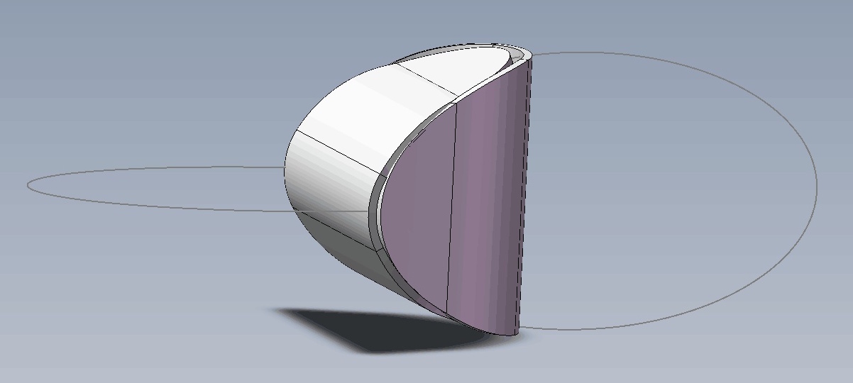
Illustration of gluing two elliptical sheets (captured from
the Zhihu question)
The problem can be expressed clearly in just a few words and can even
be understood by general readers, yet the problem itself possesses a
certain level of difficulty. This fits the criteria for a "beautiful
problem," which is why it attracted me to think about it intermittently
for several days. Finally, yesterday, I managed to provide a general equation-modeling approach and numerical
solution scheme for this type of problem, and today I completed
the theoretical proof, confirming that two
identical elliptical sheets can always be perfectly glued.
Arc Length Parametric Equation
As preparation, let us first find the arc length parametric equation
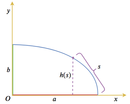
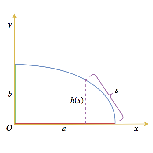
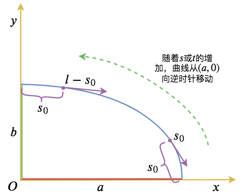
of an ellipse. As shown in the figure below, when an elliptical arc
starting from (a,0) has a length s, what is the corresponding y = h(s)?
Arc length parametric equation of an ellipse
Theoretically, this problem is not difficult to solve. Since the
standard equation of an ellipse is: \frac{x^2}{a^2} + \frac{y^2}{b^2} = 1 which
means x = a\sqrt{1 - y^2/b^2}, the arc
length of the ellipse can be expressed as: s
= \int_0^y \sqrt{1 + \left(\frac{dx}{dy}\right)^2} dy = \int_0^y
\sqrt{\frac{a^2 y^2}{b^4 - b^2 y^2} + 1} dy \label{eq:bs} This
integral can be represented using the "Incomplete
elliptic integral of the second kind". Within the interval [0, b], s is
monotonically increasing with respect to y, so an inverse function must exist. For
numerical calculation, we do not need to know the explicit form of this
inverse function; we only need to calculate a set of (y, s) correspondences through numerical
integration of [eq:bs]. By swapping the positions of y and s, we
effectively obtain the relationship y =
h(s) (defining the function point-by-point).
Equation of the Gluing Edge
Now let’s look at the original problem: assuming they can be glued,
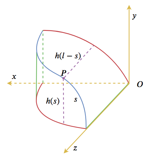
what is the equation of the edge curve? We establish a coordinate system
as shown in the figure below (left):
Arc length parametric equation of an ellipse
In the figure above, we only consider the first octant. The blue line
is the curve for which we want to find the parametric equation. The
correspondence between the spatial curve and the original elliptical
plane curve is indicated using the same colors as in the previous figure
(right). Let P = (x(s), y(s), z(s)) be
a point on the curve. Suppose the arc length OP is s;
this arc length is actually the original arc length on the ellipse. As
discussed earlier, the y-coordinate can
be found from the arc length: y = h(s)
Then, due to symmetry (complementarity), the z-coordinate is actually the y-coordinate corresponding to an arc length
of l - s, namely: z = h(l - s) where l is 1/4 of the total circumference of the
ellipse, which is the total length of the blue curve.
Now that we have y and z, we only lack x. Since s
is the arc length parameter, it must satisfy dx^2 + dy^2 + dz^2 = ds^2, i.e., \left(\frac{dx(s)}{ds}\right)^2 +
\left(\frac{dh(s)}{ds}\right)^2 + \left(\frac{dh(l-s)}{ds}\right)^2 =
1 Thus, x(s) can be integrated:
x(s) = \int_0^s \sqrt{1 -
\left(\frac{dh(s)}{ds}\right)^2 - \left(\frac{dh(l-s)}{ds}\right)^2} ds
\label{eq:f} The condition for whether they can be glued is
whether the following inequality holds constantly: 1 - \left(\frac{dh(s)}{ds}\right)^2 -
\left(\frac{dh(l-s)}{ds}\right)^2 \geq 0 \label{eq:c}
Proof of Gluing Possibility
Below we prove theoretically that two elliptical sheets can be perfectly
glued, which means verifying that [eq:c] holds
constantly.
First, we need to prove a lemma:
In an ellipse x^2/a^2 + y^2/b^2 = 1
(a \geq b > 0), we have: \left.\left(\frac{dy}{dx}\right)^2\right|_{s=s_0}
\leq \left.\left(\frac{dx}{dy}\right)^2\right|_{s=l-s_0} That is,
the absolute value of the slope at arc length s_0 does not exceed the absolute value of the
reciprocal of the slope at arc length l-s_0.
The proof process is as follows (it is not difficult; drawing it by
hand makes it clear):
Using the common parametric equations of an ellipse: x = a \cos t, \quad y = b \sin t Note that
the direction of increasing parameter t
is the same as the direction of increasing s (both counterclockwise starting from (a,0)), so s
and t have a monotonically increasing
relationship.
Intuitively, it is to prove that the "arrow on the left
viewed from the side" is steeper than the "arrow on the right viewed
from the front"
We can obtain: \left.\left(\frac{dy}{dx}\right)^2\right|_{t=t_0} =
\frac{b^2 \cos^2 t_0}{a^2 \sin^2 t_0} \leq \frac{a^2 \sin^2 (\pi/2 -
t_0)}{b^2 \cos^2 (\pi/2 - t_0)} =
\left.\left(\frac{dx}{dy}\right)^2\right|_{t=\pi/2-t_0} That is,
the slope at t=t_0 definitely does not
exceed the absolute value of the reciprocal of the slope at t=\pi/2-t_0. Obviously, the smaller t_0 is, the larger \left.\left(\frac{dx}{dy}\right)^2\right|_{t=\pi/2-t_0}
becomes.
Then we consider: \frac{ds}{dt} =
\sqrt{\left(\frac{dx}{dt}\right)^2 + \left(\frac{dy}{dt}\right)^2} =
\sqrt{a^2 \sin^2 t + b^2 \cos^2 t} = \sqrt{a^2 - (a^2 - b^2) \cos^2
t} Note that this is a monotonically increasing function of t (considering only the interval t \in [0, \pi/2]). This means s increases as t increases, and the rate of increase also
gets faster. This implies: s_{[0, t_0]} \leq
s_{[\pi/2-t_0, \pi/2]} That is, the arc length of the interval
[0, t_0] does not exceed the arc length
of the interval [\pi/2-t_0, \pi/2].
This further implies that if s_{[0, t_0]} =
s_{[\pi/2-t_1, \pi/2]}, then t_1 \leq
t_0. In other words, if s=s_0
corresponds to t=t_0 and s=l-s_0 corresponds to t=t_1, then t_1
\leq t_0. According to the previous discussion: \left.\left(\frac{dy}{dx}\right)^2\right|_{s=s_0} =
\left.\left(\frac{dy}{dx}\right)^2\right|_{t=t_0} \leq
\left.\left(\frac{dx}{dy}\right)^2\right|_{t=\pi/2-t_1} =
\left.\left(\frac{dx}{dy}\right)^2\right|_{s=l-s_0}
With this lemma, we proceed to prove: \left(\frac{dh(s)}{ds}\right)^2 +
\left(\frac{dh(l-s)}{ds}\right)^2 \leq 1 Here h(s) is the original y-coordinate of the ellipse. Suppose the
corresponding x-coordinate is g(s), then: \left(\frac{dh(s)}{ds}\right)^2 +
\left(\frac{dg(s)}{ds}\right)^2 = 1 Then it is equivalent to
proving: \left(\frac{dh(l-s)}{ds}\right)^2
\leq \left(\frac{dg(s)}{ds}\right)^2 Taking the reciprocal of
both sides and using ds^2 = dg^2 +
dh^2, it is essentially proving: \left.\left(\frac{dg}{dh}\right)^2\right|_{s=l-s_0}
\geq \left.\left(\frac{dh}{dg}\right)^2\right|_{s=s_0} This is
exactly the lemma we just proved.
Numerical Solution Results
From a mathematical perspective, [eq:f] can already
be called an explicit solution (analytical solution) for the required
curve. Of course, an explicit solution does not mean it is an elementary
function solution, nor does it mean such a solution is easy to
calculate. Although most results in differential geometry are equations
with arc length as a parameter, those are mostly theoretical. In fact,
except for circles and lines, very few curves have simple arc length
parametric equations.
To numerically verify condition [eq:c] and solve
[eq:f], I found that existing mathematical
software (like Mathematica) is not very convenient to use. The easiest
way (for me) is to write a piece of Python code to simulate the
solution. Taking a=2, b=1 as an
example, it passed the numerical verification of [eq:c] and yielded
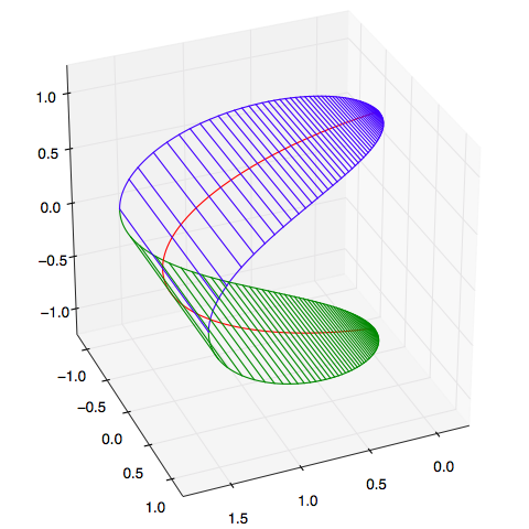
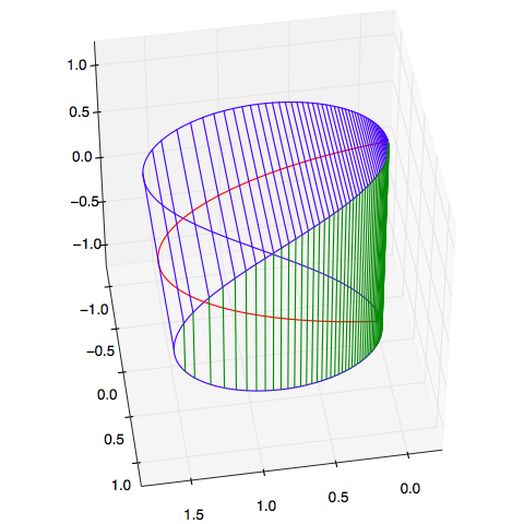
the following solution:
The curved shape of the elliptical sheets when
glued
The code is as follows:
#! -*- coding: utf-8 -*-

import numpy as np

a = 2
b = 1
h = 1e-6 # Step size

def Int(y, x):
    """Custom numerical integration function"""
    assert len(y) == len(x)
    dx = np.diff(x)
    _x = (x[:-1] + x[1:]) / 2
    _y = (y[:-1] + y[1:]) / 2
    s = np.cumsum(_y * dx)
    s = np.interp(x, _x, s, left=0)
    return s, x

def D(y, x):
    """Custom numerical differentiation function"""
    assert len(y) == len(x)
    dy = np.diff(y) + 1e-10
    dx = np.diff(x) + 1e-10
    dy_dx = dy / dx
    _x = (x[:-1] + x[1:]) / 2
    dy_dx = np.interp(x, _x, dy_dx)
    return dy_dx, x

def s2y():
    """Mapping from arc length to ellipse y-axis (i.e., h(s))"""
    y = np.arange(0, b, h)
    ds = np.sqrt(1 + a**2 * y**2 / b**2 / (b**2 - y**2))
    return Int(ds, y)[::-1]

y, s = s2y()
l = s[-1]
z = np.interp(l - s, s, y)
dx2 = 1 - D(y, s)[0]**2 - D(z, s)[0]**2
# Check if gluing is possible: whether it's >= 0 within 10x step size error
assert (dx2 > - 10 * h).all()
dx = np.sqrt(np.clip(dx2, 0, a))
x = Int(dx, s)[0]

# Sample 1/10 of the points for plotting
x = x[::10]
y = y[::10]
z = z[::10]

from mpl_toolkits.mplot3d import Axes3D
import matplotlib.pyplot as plt

plt.clf()
fig = plt.figure(figsize=(8, 8))
ax = fig.add_subplot(111, projection='3d')
ax.plot(x, y, z, color='blue')
ax.plot(x, -y, z, color='blue')
ax.plot(x, y, -z, color='green')
ax.plot(x, -y, -z, color='green')
ax.plot(x, np.zeros_like(x), z, color='red')
ax.plot(x, np.zeros_like(x), -z, color='red')

for i in range(0, len(x), 2000):
    _ = ax.plot([x[i], x[i]], [y[i], -y[i]], [z[i], z[i]], color='blue')
    _ = ax.plot([x[i], x[i]], [y[i], -y[i]], [-z[i], -z[i]], color='green')

for i in [-1, -1000]:
    _ = ax.plot([x[i], x[i]], [y[i], -y[i]], [z[i], z[i]], color='blue')
    if i != -1:
        _ = ax.plot([x[i], x[i]], [y[i], -y[i]], [-z[i], -z[i]], color='green')

ax.set_xlim(0, a)
ax.set_ylim(-b * 1.2, b * 1.2)
ax.set_zlim(-b * 1.2, b * 1.2)

plt.show()
Summary
This article analyzed the gluing problem of two elliptical sheets.
The core idea is to parameterize the curve equation using arc length.
Although the article uses an ellipse as an example, it can obviously be
generalized to the bending and gluing problem of any two general planar
curves. One only needs to find their respective arc length parametric
equations (i.e., replace h(l-s) with
the arc length parameterization of the other curve) and then use the
integral in [eq:f].
I have finally basically solved a quite interesting problem, proving
that my mathematical interest and ability are still there!