ON-LSTM: Expressing Hierarchical Structures with Ordered Neurons

Reviewing LSTM

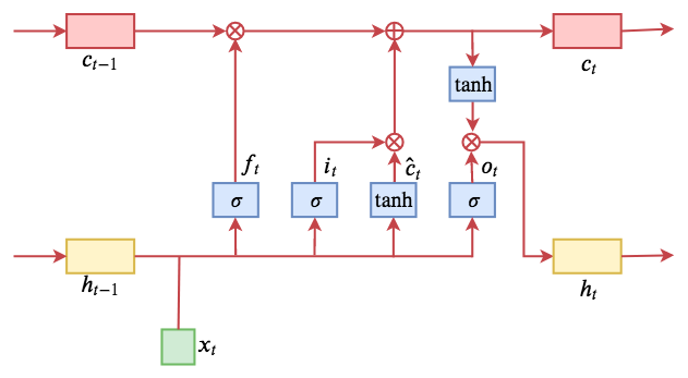
First, let’s review the standard LSTM. Using common notation, a standard LSTM is written as: \begin{aligned} f_{t} & = \sigma \left( W_{f} x_{t} + U_{f} h_{t - 1} + b_{f} \right) \\ i_{t} & = \sigma \left( W_{i} x_{t} + U_{i} h_{t - 1} + b_{i} \right) \\ o_{t} & = \sigma \left( W_{o} x_{t} + U_{o} h_{t - 1} + b_{o} \right) \\ \hat{c}_t & = \tanh \left( W_{c} x_{t} + U_{c} h_{t - 1} + b_{c} \right)\\ c_{t} & = f_{t} \circ c_{t - 1} + i_{t} \circ \hat{c}_t \\ h_{t} & = o_{t} \circ \tanh \left( c_{t} \right) \end{aligned} \label{eq:lstm} If you are familiar with neural networks, this structure is not mysterious. f_t, i_t, o_t are three single-layer fully connected models. The inputs are the historical information h_{t-1} and the current information x_t, activated by a sigmoid function. Since the result of a sigmoid is between 0 and 1, their meanings can be interpreted as "gates," specifically the forget gate, input gate, and output gate. However, I personally feel that the name "gate" is not quite appropriate; perhaps "valve" would be more fitting.

With the gates in place, x_t is integrated into \hat{c}_t, and then combined with the previous "gates" via the \circ operation (element-wise multiplication, sometimes denoted as \otimes) to perform a weighted sum of c_{t-1} and \hat{c}_t.

Below is a schematic diagram of the LSTM I drew myself:

Language and Order Information

In common neural networks, neurons are usually unordered. For example, the forget gate f_t is a vector, and the positions of the various elements in the vector have no particular pattern. If you were to shuffle the positions of all vectors involved in the LSTM operation in the same way and shuffle the weights accordingly, the output result would simply be a reordering of the original vector (in the case of multiple layers, it might even remain completely unchanged). The information content remains the same and does not affect the subsequent network’s use of it.

In other words, LSTMs and ordinary neural networks do not use the order information of neurons. ON-LSTM attempts to sort these neurons and use this order to represent specific structures, thereby utilizing the order information of the neurons.

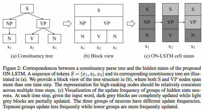
The object of study for ON-LSTM is natural language. A natural sentence can usually be represented as a hierarchical structure. If these structures are abstracted manually, they are what we call syntactic information. ON-LSTM hopes that the model can naturally learn this hierarchical structure during the training process and be able to parse it (visualize it) after training is complete. This utilizes the aforementioned neuron order information. (Related research I have done: "The Principle of Minimum Entropy (III): Sentence Templates and Language Structure").

To achieve this goal, we need a concept of levels. Lower levels represent smaller granularity structures in the language, while higher levels represent coarser granularity structures. For example, in a Chinese sentence, "characters" can be considered the lowest level structure, followed by words, and then phrases, clauses, etc. The higher the level and the coarser the granularity, the larger its span in the sentence.

Using the illustration from the original paper:

Design: Partitioned Updates

With this guidance, we can begin construction. Assuming the neurons in ON-LSTM are sorted, elements in the vector c_t with smaller indices represent lower-level information, while elements with larger indices represent higher-level information. Then, the gate structure and output structure of ON-LSTM remain the same as in a standard LSTM: \begin{aligned} f_{t} & = \sigma \left( W_{f} x_{t} + U_{f} h_{t - 1} + b_{f} \right) \\ i_{t} & = \sigma \left( W_{i} x_{t} + U_{i} h_{t - 1} + b_{i} \right) \\ o_{t} & = \sigma \left( W_{o} x_{t} + U_{o} h_{t - 1} + b_{o} \right) \\ \hat{c}_t & = \tanh \left( W_{c} x_{t} + U_{c} h_{t - 1} + b_{c} \right)\\ h_{t} & = o_{t} \circ \tanh \left( c_{t} \right) \end{aligned} \label{eq:update-o0} The difference lies in the update mechanism from \hat{c}_t to c_t.

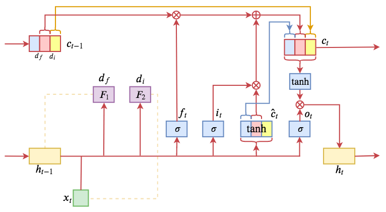
Next, initialize c_t as all zeros, meaning no memory, or imagine it as an empty USB drive. Then, we store historical information and current input into c_t according to certain rules (i.e., update c_t). Each time before updating c_t, we first predict two integers d_f and d_i, representing the levels of the historical information h_{t-1} and the current input x_t, respectively: \begin{aligned} d_f = F_1\left(x_t, h_{t-1}\right) \\ d_i = F_2\left(x_t, h_{t-1}\right) \end{aligned} As for the specific structures of F_1 and F_2, we will supplement them later; let’s clarify the core idea first. This is why I am dissatisfied with the writing of the original paper—it defines \text{cumax} right away without explaining the underlying thought before or after.

With d_f and d_i, there are two possibilities:

1. d_f \leq d_i: This means the level of the current input x_t is higher than the level of the historical record h_{t-1}. This implies that the information flows between the two intersect, and the current input information should be integrated into levels greater than or equal to d_f. The method is: \begin{aligned} c_t = \begin{pmatrix}\hat{c}_{t,< d_f} \\ f_{t,[d_f:d_i]}\circ c_{t-1,[d_f:d_i]} + i_{t,[d_f:d_i]}\circ \hat{c}_{t,[d_f:d_i]} \\ c_{t-1,> d_i} \end{pmatrix} \end{aligned} \label{eq:update-o1} This formula says that because the current input level is higher, it affects the intersection part [d_f, d_i], which is updated using the standard LSTM update formula. The part smaller than d_f is directly overwritten by the corresponding part of the current input \hat{c}_t, and the part larger than d_i keeps the corresponding part of the historical record c_{t-1} unchanged.

This update formula is intuitive because we have already sorted the neurons, with earlier positions storing lower-level structural information. For the current input, it is clearly easier to affect low-level information, so the "impact" range of the current input is [0, d_i] (bottom-up); this can also be understood as the storage space required by the current input being [0, d_i]. For the historical record, it preserves high-level information, so its "impact" range is [d_f, d_{\max}] (top-down, where d_{\max} is the highest level); perhaps we can say the storage space required by the historical information is [d_f, d_{\max}]. In the non-overlapping parts, they "govern themselves," each retaining its own information; in the overlapping part, the information must be fused, reverting to a standard LSTM.

2. d_f > d_i: This means the historical record h_{t-1} and the current input x_t do not intersect. The interval (d_i, d_f) is "unclaimed," so it remains in its initial state (all zeros, which can be understood as nothing being written). For the remaining parts, the current input writes its information directly into the [0, d_i] interval, and the historical information writes directly into the [d_f, d_{\max}] interval. In this case, the combination of current input and historical information cannot fill the entire storage space, leaving some empty capacity (the middle part is all zeros): \begin{aligned} c_t = \begin{pmatrix}\hat{c}_{t,\leq d_i} \\ 0_{(d_i : d_f)} \\ c_{t-1,\geq d_f} \end{pmatrix} \end{aligned} \label{eq:update-o2} where (d_i : d_f) denotes the interval greater than d_i and less than d_f; while the previous [d_f : d_i] denotes the interval greater than or equal to d_f and less than or equal to d_i.

At this point, we can understand the basic principle of ON-LSTM. It sorts neurons to represent the level of information hierarchy through their positions. Then, when updating neurons, it predicts the historical level d_f and the input level d_i separately, using these two levels to implement partitioned updates on the neurons.

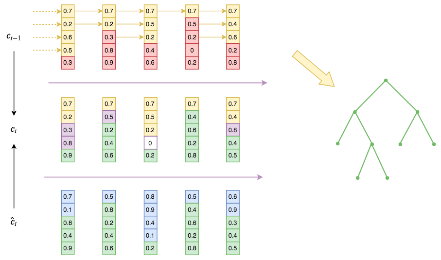
In this way, high-level information may be preserved over a considerable distance (because high-level directly copies historical information, which may be continuously copied without change), while low-level information may be updated at every input step (because low-level directly copies the input, which is constantly changing). Thus, the hierarchical structure is embedded through information grading. More simply, it is grouped updates: higher groups transmit information further (larger span), while lower groups have smaller spans. These different spans form the hierarchical structure of the input sequence.

(Please read this paragraph repeatedly, referring to the diagram above if necessary, until you fully understand it. This paragraph can be called the design manifesto of ON-LSTM.)

Formulation: Segmented Softening

The problem to solve now is how to predict these two levels, i.e., how to construct F_1 and F_2. It is not difficult to use a model to output an integer, but such models are usually non-differentiable and cannot be well-integrated into the entire model for backpropagation. Therefore, a better solution is to "soften" them, i.e., seek smooth approximations.

To perform softening, we first rewrite equations [eq:update-o1] and [eq:update-o2]. Introducing the notation 1_k, which represents a d_{\max}-dimensional vector with 1 at the k-th position and 0 elsewhere (i.e., a one-hot vector), then [eq:update-o1] and [eq:update-o2] can be unified as: \begin{aligned} \tilde{f}_t & = \stackrel{\rightarrow}{\text{cs}}\left(1_{d_f}\right), \quad \tilde{i}_t = \stackrel{\leftarrow}{\text{cs}}\left(1_{d_i}\right) \\ \omega_t & = \tilde{f}_t \circ \tilde{i}_t \quad (\text{used to represent the intersection})\\ c_t & = \underbrace{\omega_t \circ \left(f_{t} \circ c_{t - 1} + i_{t} \circ \hat{c}_t \right)}_{\text{Intersection part}} + \underbrace{\left(\tilde{f}_t - \omega_t\right)\circ c_{t - 1}}_{\text{Part greater than }\max\left(d_f, d_i\right)} + \underbrace{\left(\tilde{i}_t - \omega_t\right)\circ \hat{c}_{t}}_{\text{Part smaller than }\min\left(d_f,d_i\right)} \end{aligned} \label{eq:update-o3} where \stackrel{\rightarrow}{\text{cs}} and \stackrel{\leftarrow}{\text{cs}} are the rightward and leftward cumulative sum (cumsum) operations, respectively: \begin{aligned} \stackrel{\rightarrow}{\text{cs}}([x_1,x_2,\dots,x_n]) & = [x_1, x_1+x_2, \dots,x_1+x_2+\dots+x_n]\\ \stackrel{\leftarrow}{\text{cs}}([x_1,x_2,\dots,x_n]) & = [x_1+x_2+\dots+x_n,\dots,x_n+x_{n-1},x_n] \end{aligned} Note that the result given by [eq:update-o3] is completely equivalent to the results given by the cases in [eq:update-o1] and [eq:update-o2]. This only requires noting that \tilde{f}_t provides a d_{\max}-dimensional vector that is all 1s starting from the d_f-th position and 0s elsewhere, while \tilde{i}_t provides a d_{\max}-dimensional vector that is all 1s from position 0 to d_i and 0s elsewhere. Then \omega_t = \tilde{f}_t \circ \tilde{i}_t exactly gives a vector where the intersection part is 1 and the rest are 0 (if there is no intersection, it is an all-zero vector). Thus, \omega_t \circ \left(f_{t} \circ c_{t - 1} + i_{t} \circ \hat{c}_t \right) handles the intersection part; \left(\tilde{f}_t - \omega_t\right) yields a d_{\max}-dimensional vector that is all 1s starting from the \max\left(d_f,d_i\right)-th position, marking the range of historical information [d_f, d_{\max}] after removing the intersection; and \left(\tilde{i}_t - \omega_t\right) yields a d_{\max}-dimensional vector that is all 1s from 0 \sim \min\left(d_f,d_i\right), marking the range of current input [0, d_i] after removing the intersection.

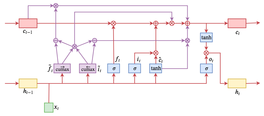
Now, the update formula for c_t is described by equation [eq:update-o3]. The two one-hot vectors 1_{d_f}, 1_{d_i} are determined by the two integers d_f, d_i, which are themselves predicted by models F_1, F_2. So we can simply have the models predict 1_{d_f}, 1_{d_i} directly. Of course, even if we predict two one-hot vectors, it doesn’t change the fact that the entire update process is non-differentiable. However, we can consider replacing 1_{d_f}, 1_{d_i} with general floating-point vectors, such as: \begin{aligned} 1_{d_f} \approx & \text{softmax}\left( W_{\tilde{f}} x_{t} + U_{\tilde{f}} h_{t - 1} + b_{\tilde{f}} \right)\\ 1_{d_i} \approx & \text{softmax}\left( W_{\tilde{i}} x_{t} + U_{\tilde{i}} h_{t - 1} + b_{\tilde{i}} \right) \end{aligned} In this way, we use a fully connected layer with h_{t-1} and x_t to predict two vectors and apply \text{softmax}, which can serve as an approximation for 1_{d_f}, 1_{d_i}. This is completely differentiable. By substituting these into [eq:update-o3], we get the update formula for c_t in ON-LSTM: \begin{aligned} \tilde{f}_t & = \stackrel{\rightarrow}{\text{cs}}\left(\text{softmax}\left( W_{\tilde{f}} x_{t} + U_{\tilde{f}} h_{t - 1} + b_{\tilde{f}} \right)\right)\\ \tilde{i}_t & = \stackrel{\leftarrow}{\text{cs}}\left(\text{softmax}\left( W_{\tilde{i}} x_{t} + U_{\tilde{i}} h_{t - 1} + b_{\tilde{i}} \right)\right) \\ \omega_t & = \tilde{f}_t \circ \tilde{i}_t \quad (\text{used to represent the intersection})\\ c_t & = \omega_t \circ \left(f_{t} \circ c_{t - 1} + i_{t} \circ \hat{c}_t \right) + \left(\tilde{f}_t - \omega_t\right)\circ c_{t - 1} + \left(\tilde{i}_t - \omega_t\right)\circ \hat{c}_{t} \end{aligned} Writing the remaining parts (i.e., [eq:update-o0]) together, the complete update formulas for ON-LSTM are: \begin{aligned} f_{t} & = \sigma \left( W_{f} x_{t} + U_{f} h_{t - 1} + b_{f} \right) \\ i_{t} & = \sigma \left( W_{i} x_{t} + U_{i} h_{t - 1} + b_{i} \right) \\ o_{t} & = \sigma \left( W_{o} x_{t} + U_{o} h_{t - 1} + b_{o} \right) \\ \hat{c}_t & = \tanh \left( W_{c} x_{t} + U_{c} h_{t - 1} + b_{c} \right)\\ \tilde{f}_t & = \stackrel{\rightarrow}{\text{cs}}\left(\text{softmax}\left( W_{\tilde{f}} x_{t} + U_{\tilde{f}} h_{t - 1} + b_{\tilde{f}} \right)\right)\\ \tilde{i}_t & = \stackrel{\leftarrow}{\text{cs}}\left(\text{softmax}\left( W_{\tilde{i}} x_{t} + U_{\tilde{i}} h_{t - 1} + b_{\tilde{i}} \right)\right) \\ \omega_t & = \tilde{f}_t \circ \tilde{i}_t\\ c_t & = \omega_t \circ \left(f_{t} \circ c_{t - 1} + i_{t} \circ \hat{c}_t \right) + \left(\tilde{f}_t - \omega_t\right)\circ c_{t - 1} + \left(\tilde{i}_t - \omega_t\right)\circ \hat{c}_{t}\\ h_{t} & = o_{t} \circ \tanh \left( c_{t} \right) \end{aligned} The schematic diagram is as follows. Comparing it with the LSTM in [eq:lstm], you can see where the main changes are. The newly introduced \tilde{f}_t and \tilde{i}_t are called the "master forget gate" and "master input gate" by the authors.

Notes:

1. In the paper, \stackrel{\rightarrow}{\text{cs}}(\text{softmax}(x)) is abbreviated as \text{cumax}(x); this is just a change in notation.

2. Viewed as a sequence, \tilde{f}_t is a monotonically increasing sequence, while \tilde{i}_t is a monotonically decreasing sequence.

3. For \tilde{i}_t, the paper defines it as: 1 - \text{cumax}\left( W_{\tilde{i}} x_{t} + U_{\tilde{i}} h_{t - 1} + b_{\tilde{i}} \right) This choice produces a similar monotonically decreasing vector. In general, there is no difference, but from the perspective of symmetry, I believe my choice is more reasonable.

Grouping Levels

The vectors \tilde{f}_t, \tilde{i}_t representing levels must undergo the \circ operation with f_t, etc., which means their dimensions (i.e., the number of neurons) must be equal. As we know, depending on the requirements, the number of hidden neurons in an LSTM can reach several hundred or even thousands, which means the number of levels described by \tilde{f}_t, \tilde{i}_t would also be several hundred or thousands. In fact, the total number of levels in a sequence’s hierarchical structure (if it exists) is generally not that large, meaning there is a slight contradiction between the two.

The authors of ON-LSTM came up with a reasonable solution: assume the number of hidden neurons is n, which can be decomposed as n=pq. Then we can construct \tilde{f}_t, \tilde{i}_t with only p neurons, and then repeat each neuron of \tilde{f}_t, \tilde{i}_t exactly q times to obtain an n-dimensional \tilde{f}_t, \tilde{i}_t, which is then used in the \circ operation with f_t, etc. For example, if n=6=2\times 3, we first construct a 2D vector like [0.1, 0.9], and then repeat each element 3 times to get [0.1, 0.1, 0.1, 0.9, 0.9, 0.9].

In this way, we both reduce the total number of levels and reduce the number of model parameters, because p can usually be taken to be quite small (1 to 2 orders of magnitude smaller than n). Therefore, compared to a standard LSTM, ON-LSTM does not add too many parameters.

Language Modeling

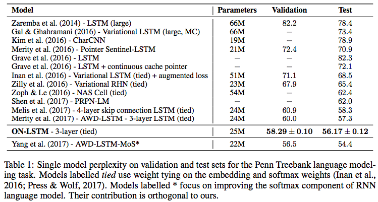
The authors conducted several experiments, including language modeling, syntactic evaluation, and logical reasoning. In many experiments, they achieved state-of-the-art results, generally surpassing standard LSTMs. This proves that the hierarchical structure information introduced by ON-LSTM is valuable. Among these, I am only familiar with language modeling, so I will just post a screenshot of the language modeling experiment results:

Unsupervised Syntax

If it only outperformed standard LSTMs in conventional language tasks, ON-LSTM might not be considered a breakthrough. However, an exciting feature of ON-LSTM is its ability to extract the hierarchical tree structure of input sequences unsupervised from a trained model (such as a language model). The extraction idea is as follows:

First, we consider: p_f = \text{softmax}\left( W_{\tilde{f}} x_{t} + U_{\tilde{f}} h_{t - 1} + b_{\tilde{f}} \right) This is the result before the \stackrel{\rightarrow}{\text{cs}} operation for \tilde{f}_t. According to our previous derivation, it is a softened version of the historical information level d_f. Thus, we can write: d_f \approx \mathop{\text{argmax}}_{k} p_f(k) where p_f(k) refers to the k-th element of the vector p_f. However, the \text{softmax} contained in p_f is itself a "softened" operator. In this case, we might consider a "softened" \text{argmax} (refer to "A Talk on Function Smoothing: Differentiable Approximation of Non-differentiable Functions"), namely: d_f \approx \sum_{k=1}^n k \times p_f(k) = n\left(1 - \frac{1}{n}\sum_{k=1}^n \tilde{f}_t(k)\right) + 1 The second equals sign is an identity transformation; you can prove it yourself (Equation (15) in the original paper is incorrect). Thus, we have obtained a formula for calculating the level. When n is fixed, it depends directly on \left(1 - \frac{1}{n}\sum\limits_{k=1}^n \tilde{f}_t(k)\right).

Consequently, we can use the sequence: \left\{d_{f,t}\right\}_{t=1}^{\text{seq\_len}} = \left\{\left(1 - \frac{1}{n}\sum\limits_{k=1}^n \tilde{f}_t(k)\right)\right\}_{t=1}^{\text{seq\_len}} to represent the level changes of the input sequence. With this level sequence, we can extract the hierarchical structure using the following greedy algorithm:

Given an input sequence \{x_t\} to a pre-trained ON-LSTM, output the corresponding level sequence \{d_{f,t}\}. Then find the index of the maximum value in the level sequence, say k. Partition the input sequence into [x_{t < k}, [x_k, x_{t > k}]]. Repeat this process recursively for the subsequences x_{t < k} and x_{t > k} until each subsequence has a length of 1.

The algorithm essentially means breaking at the highest level (which means this point contains the least historical information and has the weakest connection with all previous content, making it the most likely start of a new sub-structure) and processing recursively to gradually obtain the nested structure implicit in the input sequence. The authors trained a language model with a three-layer ON-LSTM and used the \tilde{f}_t of the middle layer to calculate levels. Comparing this with annotated syntactic structures, they found the accuracy to be quite high. I also tried it on a Chinese corpus: https://github.com/bojone/on-lstm/blob/master/lm_model.py

As for the effect, since I have not done syntactic analysis and do not understand it well, I don’t know how to evaluate it. It seems like it’s doing something right, but also seems a bit off. I’ll let the readers judge for themselves. In the last year or two, there has been quite a bit of research on unsupervised syntactic analysis; one might need to read them all to understand ON-LSTM more deeply.

Input: What is the color of the apple
Output:
[


’apple’,
’s’
,

’color’,
’is’

,
’what’
]

Input: Love really needs courage
Output:
[
’Love’,

’really’,

’needs’,
’courage’


]

Reflections and Divergence

At the end of the article, let’s think about a few questions together.

Is there still research value in RNNs?

First, some readers might be confused: it’s 2019, and people are still researching RNN-type models? Is there still research value? In recent years, pre-trained models based on Attention and language models, such as BERT and GPT, have improved performance on many NLP tasks, and some articles even say "RNN is dead." Is this really the case? I believe RNNs are alive and well and will not die for a long time, for at least several reasons:

First, models like BERT improve performance by only one or two percentage points at the cost of several orders of magnitude more computing power. This kind of cost-performance ratio is only valuable in academic research and competition leaderboards; it is almost useless in engineering (at least it cannot be used directly). Second, RNN-type models themselves have some incomparable advantages, such as easily simulating a counting function; in many sequence analysis scenarios, RNNs perform very well. Third, almost all seq2seq models (even in BERT) use some form of RNN for the decoder because they are basically recursive decoding; how could RNNs disappear?

Is a unidirectional ON-LSTM enough?

Then, readers might have doubts: you want to extract hierarchical structures, but you only used a unidirectional ON-LSTM. This means the current level analysis does not depend on future inputs, which is clearly not entirely consistent with reality. I have the same confusion, but the authors’ experiments show that this is already good enough. It may be that the overall structure of natural language tends to be local and unidirectional (from left to right), so unidirectional is sufficient for natural language.

In general cases, would bidirectional be better? If bidirectional, should it be trained using a masked language model like BERT? How would the level sequence be calculated for bidirectional? There are no complete answers to all of this yet. As for whether the unsupervised extracted structure necessarily conforms to the hierarchical structure understood by humans, that is also uncertain. Since there is no supervised guidance, the neural network "understands it in its own way." Fortunately, the neural network’s "own way" seems to have significant overlap with the human way.

Why consider d_f instead of d_i when extracting levels?

Readers might be confused: there are clearly two master gates, so why use d_f instead of d_i to extract levels? To answer this, we must understand the meaning of d_f. We said d_f is the level of historical information; in other words, it tells us how much historical information to use to make the current decision. If d_f is very large, it means the current decision uses almost no historical information, which implies that a new level starts from here, almost cutting off the connection with historical input. It is from this disconnection and connection that the hierarchical structure is extracted, so only d_f can be used.

Can this be applied to CNNs or Attention?

Finally, a possible confusion is whether this design can be used in CNNs or Attention. In other words, can the neurons of CNNs and Attention also be sorted to integrate hierarchical structure information? Personally, I feel it is possible, but it would require redesigning because hierarchical structures are assumed to be continuously nested. The recursive nature of RNNs is well-suited to describe this continuity, while the non-recursive nature of CNNs and Attention makes it difficult to directly express such continuous nested structures.

Regardless, I think this is a topic worth thinking about. I will share any further thoughts with you, and of course, readers are welcome to share their thoughts with me.