From DCGAN to SELF-MOD: An Overview of GAN Architecture Evolution

Basic Background

As is well known, GANs originated from Ian Goodfellow’s paper "Generative Adversarial Networks", but early GANs were limited to simple datasets like MNIST. This was because GANs had just emerged, and although they piqued interest, they were still in the trial-and-error stage, with issues regarding model architecture, stability, and convergence still being explored. The emergence of DCGAN laid a solid foundation for solving these problems.

DCGAN comes from the paper "Unsupervised Representation Learning with Deep Convolutional Generative Adversarial Networks". To say what it did is simple: it proposed an architecture for the generator and discriminator that greatly stabilized GAN training, to the point that it became the standard GAN architecture for a long time.

It sounds simple, but in fact, achieving this was not easy because there are many intuitively "reasonable" architectures. Screening out the nearly optimal one from various combinations clearly required a considerable number of experiments. Because DCGAN almost established the standard architecture for GANs, researchers could focus more on a wider variety of tasks without worrying too much about model architecture and stability, leading to the flourishing development of GANs.

Architecture Description

Having said all that, let’s return to the discussion of the architecture itself. The model architecture proposed by DCGAN is roughly as follows:

1. Neither the generator nor the discriminator uses pooling layers; instead, they use (strided) convolutional layers. The discriminator uses regular convolution (Conv2D), while the generator uses transposed convolution (DeConv2D).

2. Batch Normalization is used in both the generator and the discriminator.

3. The ReLU activation function is used in all layers of the generator except for the output layer, which uses the Tanh activation function.

4. The LeakyReLU activation function is used in all layers of the discriminator.

5. No fully connected layers are used after the convolutional layers.

6. Global Pooling is not used after the last convolutional layer of the discriminator; instead, it is directly flattened.

In hindsight, this is still a relatively simple structure, embodying the beauty of simplicity and further proving that good things are necessarily concise.

The schematic diagram of the DCGAN structure is as follows:

Personal Summary

Key points:

• The kernel size for convolution and transposed convolution is 4x4 or 5x5.

• The stride for convolution and transposed convolution is generally set to 2.

• For the discriminator, BN is generally not used after the first convolutional layer, and the subsequent layers follow the "Conv2D + BN + LeakyReLU" pattern until the feature map size is 4x4.

• For the generator, the first layer is fully connected, then reshaped to 4x4, followed by the "Conv2D + BN + ReLU" pattern. The last convolutional layer does not use BN and uses Tanh activation instead. Correspondingly, input images should be scaled to between -1 and 1 by dividing by 255, multiplying by 2, and subtracting 1.

Although the number of parameters might seem large, DCGAN is actually very fast and does not consume much VRAM, making it very popular. Therefore, despite being old, it is still used in many tasks today. At least for rapid experimentation, it is an excellent architecture.

Problems with DCGAN

A common saying is that because the DCGAN generator uses transposed convolution, it inherently suffers from "Checkerboard Artifacts," which limit the upper bound of DCGAN’s generative capabilities. For details on checkerboard artifacts, please refer to "Deconvolution and Checkerboard Artifacts" (highly recommended, with many visual examples).

To be precise, checkerboard artifacts are not a problem with transposed convolution itself, but an inherent flaw of stride > 1, which prevents the convolution from covering the entire image "isotropically," resulting in an interleaved effect like a chessboard. Since transposed convolution is usually paired with stride > 1, it is often blamed. In fact, besides transposed convolution, dilated convolution also exhibits checkerboard artifacts because it can be proven that dilated convolution is equivalent to regular convolution with stride > 1 under certain transformations.

On the other hand, I estimate there is another reason: the non-linear capability of DCGAN might be insufficient. Readers who have analyzed DCGAN results will notice that once the input image size is fixed, the entire DCGAN architecture is basically fixed, including the number of layers. The only thing that seems changeable is the kernel size (channel numbers can be adjusted slightly, but the room for adjustment is small). Changing the kernel size can change the non-linear capability to some extent, but it only changes the width of the model, and for deep learning, depth may be more important than width. The problem is that for DCGAN, there is no natural and direct way to increase depth.

ResNet Model

Due to the reasons above, and as ResNet became increasingly dominant in classification problems, it was natural to consider applying the ResNet structure to GANs. In fact, the mainstream generator and discriminator architectures in GANs have indeed shifted to ResNet. The basic structure is illustrated below:

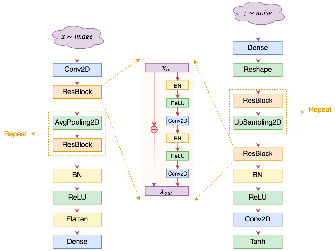
As can be seen, ResNet-based GANs do not differ significantly from DCGAN in overall structure (which further confirms the foundational role of DCGAN). The main features are:

1. In both the discriminator and generator, transposed convolutions are removed, leaving only regular convolutional layers.

2. The kernel size is usually unified to 3x3, and convolutions form residual blocks.

3. Upsampling and downsampling are achieved through AvgPooling2D and UpSampling2D, whereas in DCGAN, they were achieved through convolution/transposed convolution with stride > 1. UpSampling2D is equivalent to magnifying the image’s length/width by a certain factor.

4. Since there are already residuals, the activation function can be unified to ReLU. Of course, some models still use LeakyReLU; the difference is not significant.

5. By increasing the number of convolutional layers in the ResBlock, both the non-linear capability and the depth of the network can be increased, which is where the flexibility of ResNet lies.

6. Generally, the residual form is x + f(x), where f represents a combination of convolutional layers. However, in GANs, model initialization is generally smaller than in conventional classification models. For stability, some models change it to x + \alpha \times f(x), where \alpha is a number less than 1, such as 0.1, to achieve better stability.

7. Some authors believe BN is not suitable for GANs and sometimes remove it or replace it with LayerNorm, etc.

Personal Summary

I haven’t carefully researched which paper first used ResNet in GANs, but I know that famous GANs like PGGAN, SNGAN, and SAGAN have all adopted ResNet. The stride in ResNet is always 1, so it is uniform enough and does not produce checkerboard artifacts.

However, ResNet is not without its drawbacks. Although ResNet does not increase the number of parameters compared to DCGAN (in some cases, it even has fewer), ResNet is much slower than DCGAN and requires much more VRAM. This is because ResNet has more layers and more connections between layers, leading to more complex gradients and weaker parallelism (convolutions in the same layer can be parallelized, but convolutions in different layers are serial and cannot be directly parallelized). The result is that it is slower and more memory-intensive.

Also, checkerboard artifacts are actually a very subtle effect, perhaps only noticeable in high-definition image generation. In my experiments, doing 128x128 or even 256x256 face or LSUN generation showed no obvious visual difference between DCGAN and ResNet, but DCGAN’s speed was more than 50% faster than ResNet. In terms of VRAM, DCGAN can directly handle 512x512 generation (on a single 1080ti), while ResNet is somewhat strained even at 256x256.

Therefore, unless I need to compete for the current optimal FID or other metrics, I would not choose the ResNet architecture.

Conditional BN

Before introducing SELF-MOD, I need to introduce something else: Conditional Batch Normalization (Conditional BN).

As is well known, BN is a common operation in deep learning, especially in the image field. To be honest, I don’t like BN much, but I must admit it plays an important role in many GAN models. Regular BN is unconditional: for an input tensor \boldsymbol{x}_{i,j,k,l}, where i,j,k,l represent the batch, height, width, and channel dimensions of the image, respectively, the training phase is: \boldsymbol{x}_{i,j,k,l}^{(out)}=\boldsymbol{\gamma}_l \times \frac{\boldsymbol{x}_{i,j,k,l}^{(in)} - \boldsymbol{\mu}_l}{\boldsymbol{\sigma}_l+\epsilon} + \boldsymbol{\beta}_l where \boldsymbol{\mu}_l = \frac{1}{N}\sum_{i,j,k} \boldsymbol{x}_{i,j,k,l}^{(in)},\quad \boldsymbol{\sigma}^2_l = \frac{1}{N}\sum_{i,j,k} \left(\boldsymbol{x}_{i,j,k,l}^{(in)}-\boldsymbol{\mu}_l\right)^2 are the mean and variance of the input batch data, where N = \text{batch\_size} \times \text{height} \times \text{width}, \boldsymbol{\beta}, \boldsymbol{\gamma} are trainable parameters, and \epsilon is a small positive constant to prevent division by zero. In addition, a set of moving average variables \hat{\boldsymbol{\mu}}, \hat{\boldsymbol{\sigma}}^2 is maintained for use during the testing phase.

The reason this BN is called unconditional is that the parameters \boldsymbol{\beta}, \boldsymbol{\gamma} are obtained purely through gradient descent and do not depend on the input. Correspondingly, if \boldsymbol{\beta}, \boldsymbol{\gamma} depend on some input \boldsymbol{y}, it is called Conditional BN: \boldsymbol{x}_{i,j,k,l}^{(out)}=\boldsymbol{\gamma}_l(\boldsymbol{y}) \times \frac{\boldsymbol{x}_{i,j,k,l}^{(in)} - \boldsymbol{\mu}_l}{\boldsymbol{\sigma}_l+\epsilon} + \boldsymbol{\beta}_l(\boldsymbol{y}) In this case, \boldsymbol{\beta}_l(\boldsymbol{y}) and \boldsymbol{\gamma}_l(\boldsymbol{y}) are outputs of some model.

Let’s talk about how to implement it. In Keras, implementing Conditional BN is very easy. Refer to the following code:

def ConditionalBatchNormalization(x, beta, gamma):
    """To implement Conditional BN, we only need to remove the 
    beta and gamma from Keras's built-in BatchNormalization 
    and then pass in the external beta and gamma. For training 
    stability, beta should ideally be initialized to all zeros 
    and gamma to all ones.
    """
    x = BatchNormalization(center=False, scale=False)(x)
    def cbn(x):
        x, beta, gamma = x
        for i in range(K.ndim(x)-2):
            # Adjust the ndim of beta; modify this based on the situation
            beta = K.expand_dims(beta, 1)
            gamma = K.expand_dims(gamma, 1)
        return x * gamma + beta
    return Lambda(cbn)([x, beta, gamma])

SELF-MOD GAN

Conditional BN first appeared in the paper "Modulating early visual processing by language" and was later used in "cGANs With Projection Discriminator". It has now become the standard solution for Conditional GANs (cGANs), including SAGAN and BigGAN. Simply put, cGAN uses the label \boldsymbol{c} as the condition for \boldsymbol{\beta}, \boldsymbol{\gamma}, forming Conditional BN to replace the unconditional BN of the generator. That is, the main input of the generator is still random noise \boldsymbol{z}, and the condition \boldsymbol{c} is passed into every BN of the generator.

So what does Conditional BN have to do with SELF-MOD?

The situation is this: SELF-MOD considers that cGAN training is more stable, but in general, GANs do not have labels \boldsymbol{c} available. What to do? Just use the noise \boldsymbol{z} itself as the label! This is the meaning of Self-Modulated: regulating itself without relying on external labels, but achieving a similar effect. Described by a formula: \boldsymbol{x}_{i,j,k,l}^{(out)}=\boldsymbol{\gamma}_l(\boldsymbol{z}) \times \frac{\boldsymbol{x}_{i,j,k,l}^{(in)} - \boldsymbol{\mu}_l}{\boldsymbol{\sigma}_l+\epsilon} + \boldsymbol{\beta}_l(\boldsymbol{z}) In the original paper, \boldsymbol{\beta}(\boldsymbol{z}) is a two-layer fully connected network: \boldsymbol{\beta}(\boldsymbol{z})=\boldsymbol{W}^{(2)}\max\left(0, \boldsymbol{W}^{(1)}\boldsymbol{z}+\boldsymbol{b}^{(2)}\right) \boldsymbol{\gamma}(\boldsymbol{z}) is the same. Looking at the official source code, the dimension of the hidden layer can be quite small, such as 32, so it won’t significantly increase the number of parameters.

This is the SELF-MOD structure generator for unconditional GANs.

Personal Summary

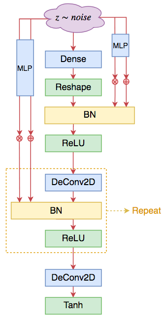
I experimented with the SELF-MOD structure in combination with my own O-GAN and found that the convergence speed increased by nearly 50%, and the final FID and reconstruction effects were better. The excellence of SELF-MOD is evident, and I have a faint feeling that O-GAN and SELF-MOD are a better match (haha, I don’t know if it’s just a narcissistic delusion).

Keras reference code: https://github.com/bojone/o-gan/blob/master/o_gan_celeba_sm_4x4.py

Additionally, even in cGAN, the SELF-MOD structure can be used. Standard cGAN uses the condition \boldsymbol{c} as the BN input condition, while SELF-MOD uses both \boldsymbol{z} and \boldsymbol{c} as BN input conditions. A reference usage is as follows: \begin{aligned} \boldsymbol{\beta}(\boldsymbol{z},\boldsymbol{c}) &= \boldsymbol{W}^{(2)}\max\left(0, \boldsymbol{W}^{(1)}\boldsymbol{z}'+\boldsymbol{b}^{(2)}\right)\\ \boldsymbol{z}' &= \boldsymbol{z}+\text{E}(\boldsymbol{c})+\text{E}'(\boldsymbol{c})\otimes \boldsymbol{z} \end{aligned} where \text{E}, \text{E}' are two Embedding layers. If the number of categories is small, they can be understood directly as fully connected layers. \boldsymbol{\gamma} is handled similarly.

AdaIN

The core of StyleGAN is something called AdaIN (Adaptive Instance Normalization), which comes from the style transfer paper "Arbitrary Style Transfer in Real-time with Adaptive Instance Normalization". It is actually similar to Conditional BN, even simpler: \boldsymbol{x}_{i,j,k,l}^{(out)}=\boldsymbol{\gamma}_l(\boldsymbol{y}) \times \frac{\boldsymbol{x}_{i,j,k,l}^{(in)} - \boldsymbol{\mu}_{i,l}}{\boldsymbol{\sigma}_{i,l}+\epsilon} + \boldsymbol{\beta}_l(\boldsymbol{y}) The difference from Conditional BN is: Conditional BN uses \boldsymbol{\mu}_l and \boldsymbol{\sigma}_l, while AdaIN uses \boldsymbol{\mu}_{i,l} and \boldsymbol{\sigma}_{i,l}. That is, AdaIN only calculates statistical features within a single sample, without needing a batch of samples. Therefore, AdaIN does not need to maintain moving average means and variances, making it simpler than Conditional BN.

StyleGAN

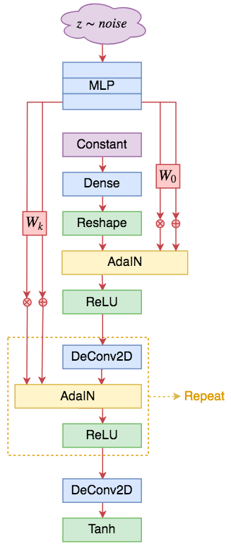
With SELF-MOD and AdaIN, StyleGAN can be explained clearly. The main change in StyleGAN is also the generator. Compared to SELF-MOD, its differences are:

1. Cancel the noise input at the top and replace it with a trainable constant vector.

2. Replace all Conditional BNs with AdaIN.

3. The input condition for AdaIN is the noise transformed by a multi-layer MLP, then projected by different transformation matrices into \boldsymbol{\beta} and \boldsymbol{\gamma} for different AdaIN layers.

It’s that simple!

Personal Summary

I also experimented with a simplified StyleGAN-style DCGAN and found that it could converge and the results were okay, but there was slight Mode Collapse. Since the official StyleGAN was trained using the PGGAN mode and I didn’t use it, I wonder if StyleGAN needs to be paired with PGGAN to be trained well? There is no answer yet. It’s just that in my experiments, SELF-MOD was much easier to train than StyleGAN and yielded better results.