In this post, I would like to share a recent piece of work: by simply modifying the original GAN model, the discriminator can be transformed into an encoder. This allows the GAN to possess both generative and encoding capabilities simultaneously, with almost no increase in training cost. This new model is called O-GAN (Orthogonal GAN), as it is based on an orthogonal decomposition of the discriminator, representing the most efficient utilization of the discriminator’s degrees of freedom.
Arxiv Link: https://papers.cool/arxiv/1903.01931
Open Source Code: https://github.com/bojone/o-gan
Background
I have been immersed in the field of generative models for a long time. Not only have I written numerous blog posts about them, but I have also submitted several small papers related to generative models to Arxiv. Since diving into this area, although my understanding of generative models—especially GANs—has deepened, and I sometimes felt I made improvements (hence the Arxiv submissions), the truth is that those works were mostly minor tweaks of little significance.
However, I believe the model introduced in this article is more valuable than the sum of all my previous GAN-related work: it provides the simplest solution currently available to train a GAN model with encoding capabilities.
Nowadays, GANs have become increasingly mature and massive. State-of-the-art models like BigGAN and StyleGAN are well-known and widely used. However, these advanced GAN models currently only function as generators; they lack an encoder, meaning they can generate an endless stream of new images but cannot extract features from existing ones.
Of course, there has been research into GANs with encoders, and I have even explored this on this blog (refer to "BiGAN-QP: A Simple and Clear Encoding & Generative Model"). But regardless of whether they have encoding capabilities, most GANs share a common trait: after training is complete, the discriminator is useless. This is because, theoretically, as training progresses, the discriminator degrades (e.g., it tends toward a constant).
Anyone who has worked with GANs knows that the complexity of the discriminator and the generator is comparable (and if there is an encoder, its complexity is similar as well). Discarding the discriminator after training is a serious waste of such a large network! Generally, the architecture of a discriminator is very similar to that of an encoder. A natural thought is: can the discriminator and encoder share most of their weights? To my knowledge, among all past GAN-related models, only IntroVAE achieved this. However, IntroVAE’s approach is relatively complex, and there is currently no successful open-source replication of IntroVAE available online (I attempted to replicate it myself and failed).
The solution in this article is extremely simple—by slightly modifying the original GAN model, the discriminator can be converted into an encoder, with almost no increase in complexity or computational overhead.
Model
Without further ado, let’s introduce the model. First, we introduce the general GAN formulation: \begin{aligned} D &= \mathop{\text{argmin}}_{D} \mathbb{E}_{x\sim p(x), z\sim q(z)}\Big[f(D(x)) + g(D(G(z)))\Big] \\ G &= \mathop{\text{argmin}}_{G} \mathbb{E}_{z\sim q(z)}\Big[h(D(G(z)))\Big] \end{aligned} To avoid confusion, I will define the symbols clearly. Here x\in \mathbb{R}^{n_x}, z\in \mathbb{R}^{n_z}, p(x) is the "evidence distribution" of the real image set, and q(z) is the noise distribution (in this article, it is an n_z-dimensional standard normal distribution). G: \mathbb{R}^{n_z} \to \mathbb{R}^{n_x} and D: \mathbb{R}^{n_x} \to \mathbb{R} are the generator and discriminator, respectively. f, g, h are specific functions; different GANs correspond to different f, g, h. Sometimes we add normalization or regularization methods, such as spectral normalization or gradient penalty; for simplicity, these are not explicitly written out.
Next, we define several vector operators: \text{avg}(z)=\frac{1}{n_z}\sum_{i=1}^{n_z} z_i,\quad \text{std}(z)=\sqrt{\frac{1}{n_z}\sum_{i=1}^{n_z} (z_i-\text{avg}(z))^2}, \quad \mathcal{N}(z)=\frac{z - \text{avg}(z)}{\text{std}(z)} While these look sophisticated, they are simply the mean, standard deviation, and the standardized version of the vector’s elements. Notably, when n_z \geq 3 (which is true for all valuable GANs), [\text{avg}(z), \text{std}(z), \mathcal{N}(z)] is functionally independent, meaning it acts as an "orthogonal decomposition" of the original vector z.
As mentioned, the discriminator’s structure is similar to an encoder, except that an encoder outputs a vector while a discriminator outputs a scalar. Thus, we can write the discriminator as a composite function: D(x) \triangleq T(E(x)) Here E is a mapping from \mathbb{R}^{n_x} \to \mathbb{R}^{n_z}, and T is a mapping from \mathbb{R}^{n_z} \to \mathbb{R}. It is easy to imagine that the number of parameters in E will far exceed those in T. We want E(x) to function as an encoder.
How do we achieve this? We simply add a loss: the Pearson correlation coefficient! \begin{aligned} T,E &= \mathop{\text{argmin}}_{T,E} \mathbb{E}_{x\sim p(x), z\sim q(z)}\Big[f(T(E(x))) + g(T(E(G(z)))) - \lambda \rho(z, E(G(z)))\Big] \\ G &= \mathop{\text{argmin}}_{G} \mathbb{E}_{z\sim q(z)}\Big[h(T(E(G(z)))) - \lambda \rho(z, E(G(z)))\Big] \end{aligned} where \rho(z, \hat{z})=\frac{\sum\limits_{i=1}^{n_z} (z_i - \text{avg}(z))(\hat{z}_i - \text{avg}(\hat{z}))/n_z}{\text{std}(z)\times \text{std}(\hat{z})}=\cos(\mathcal{N}(z), \mathcal{N}(E(G(z))))
If \lambda=0, it is just a standard GAN (with the discriminator decomposed into E and T). By adding this correlation coefficient, we intuitively hope that z and E(G(z)) are as linearly correlated as possible. Why add it this way? We will discuss that at the end.
Clearly, this correlation coefficient can be embedded into any existing GAN with minimal changes (splitting the discriminator and adding a loss). I have experimented with various GANs and found that all can be trained successfully.
In this setup, the GAN discriminator D is divided into E and T, and E becomes the encoder. This means most of the discriminator’s parameters are utilized. However, T remains; after training, T is still useless. Although T has few parameters and the waste is minimal, it is still bothersome for "perfectionists" (like myself).
Can we eliminate T as well? After multiple trials, the conclusion is: yes, we can! We can directly use \text{avg}(E(x)) as the discriminator: \begin{aligned} E &= \mathop{\text{argmin}}_{E} \mathbb{E}_{x\sim p(x), z\sim q(z)}\Big[f(\text{avg}(E(x))) + g(\text{avg}(E(G(z)))) - \lambda \rho(z, E(G(z)))\Big] \\ G &= \mathop{\text{argmin}}_{G} \mathbb{E}_{z\sim q(z)}\Big[h(\text{avg}(E(G(z)))) - \lambda \rho(z, E(G(z)))\Big] \end{aligned} \label{eq:simplest} Now the entire model has no T, only the pure generator G and encoder E. There is no redundancy in the model at all.
Experiments
Why does this work? We’ll discuss that later. First, let’s look at the experimental results. After all, if the experiments aren’t good, the theory is meaningless.
Note that theoretically, the correlation coefficient term introduced here does not improve the quality of the generative model. Therefore, the experiments have two main goals: 1. Does this extra loss harm the quality of the original generative model? 2. Does this extra loss truly turn E into an effective encoder?
As mentioned, this method can be embedded into any GAN. For this experiment, I used a variant of my previous GAN-QP: \begin{aligned} E &= \mathop{\text{argmin}}_{E} \mathbb{E}_{x\sim p(x), z\sim q(z)}\Big[\text{avg}(E(x)) - \text{avg}(E(G(z))) + \lambda_1 R_{x,z} - \lambda_2 \rho(z, E(G(z)))\Big] \\ G &= \mathop{\text{argmin}}_{G} \mathbb{E}_{z\sim q(z)}\Big[\text{avg}(E(G(z))) - \lambda_2 \rho(z, E(G(z)))\Big] \end{aligned} \label{eq:simplest-2} where R_{x,z} = \frac{[\text{avg}(E(x)) - \text{avg}(E(G(z)))]^2}{\Vert x - G(z)\Vert^2}
Regarding datasets, the experiments were quite comprehensive, covering CelebA HQ, FFHQ, LSUN-churchoutdoor, and LSUN-bedroom, all at 128\times 128 resolution (I also did some 256\times 256 experiments with good results, but they weren’t included in the paper). The model architecture is the same DCGAN as before; for other details, please refer to the paper or the code.
Images:
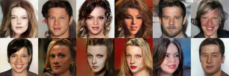
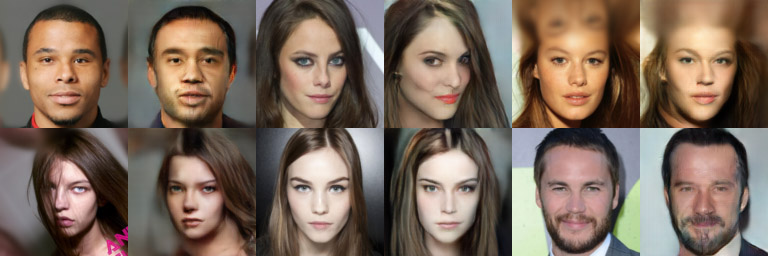
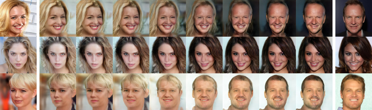
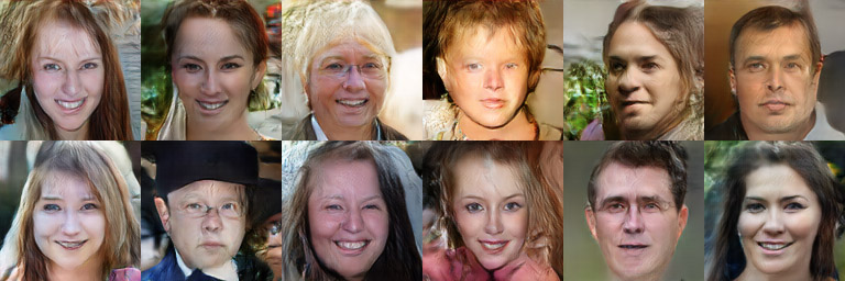
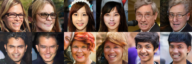
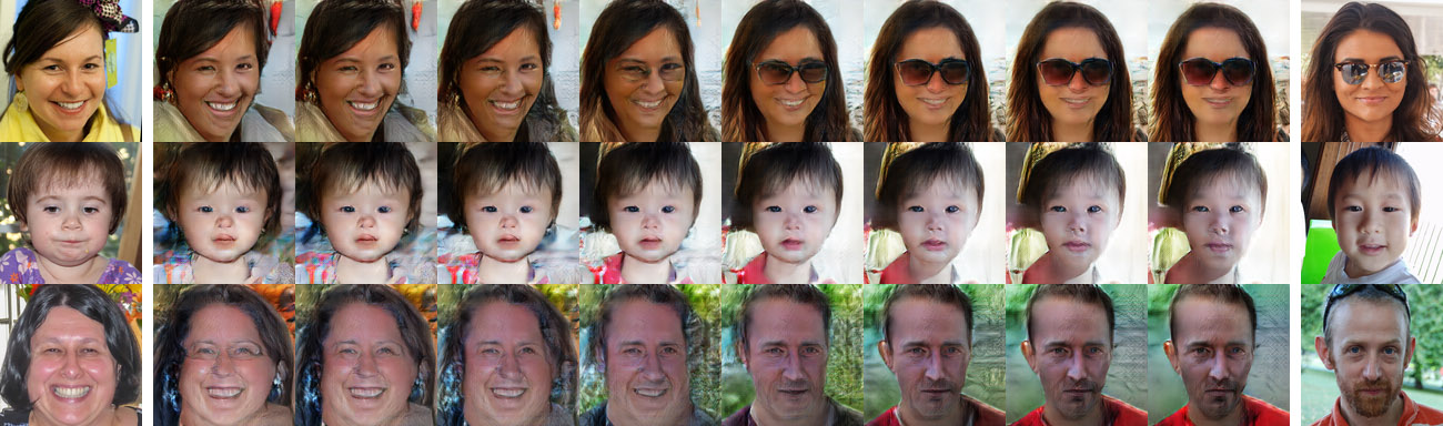
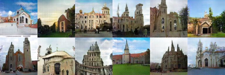

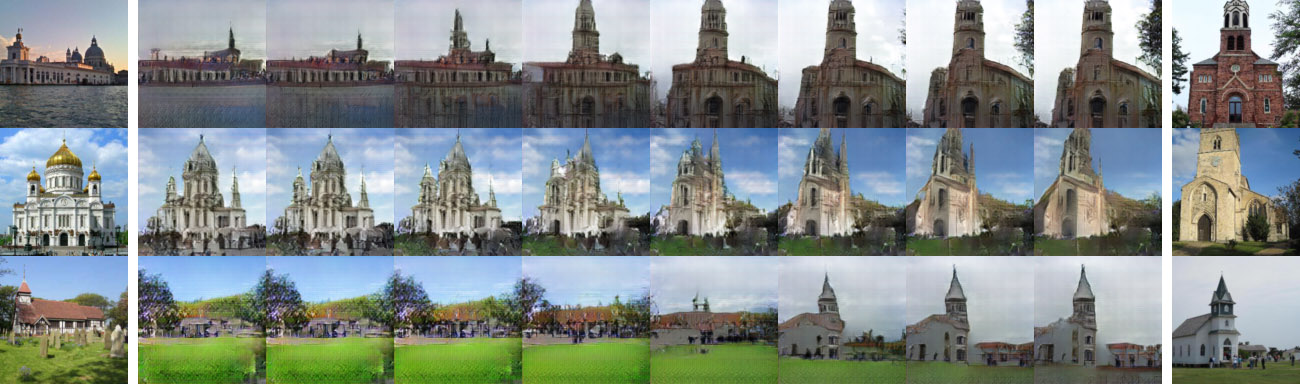
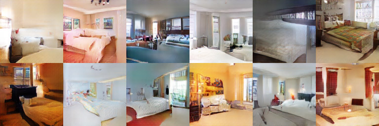

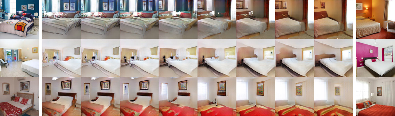
Whether you think they are good or not, I personally find them quite satisfactory.
Random generation results are good, indicating the new correlation term does not degrade generation quality.
Reconstruction results are good, indicating E(x) indeed extracts the main features of x.
Linear interpolation results are good, indicating E(x) has learned features that are nearly linearly separable.
Principle
Now that the results are confirmed, let’s discuss the principle.
Obviously, the role of this extra reconstruction term is to make z as "correlated" as possible with E(G(z)). For this, most readers’ first thought might be the MSE loss \Vert z - E(G(z))\Vert^2 rather than the \rho(z, E(G(z))) used here. However, if \Vert z - E(G(z))\Vert^2 is used, the training will almost certainly fail. Why does \rho(z, E(G(z))) succeed?
According to the previous definition, E(x) outputs an n_z-dimensional vector, but T(E(x)) outputs only a scalar. This means E(x) provides n_z degrees of freedom, and as a discriminator, T(E(x)) must occupy at least one degree of freedom (theoretically, it only needs one). If we minimize \Vert z - E(G(z))\Vert^2, the training process forces E(G(z)) to be exactly equal to z, meaning all n_z degrees of freedom are occupied by it, leaving no degrees of freedom for the discriminator to distinguish between real and fake. Thus, adding \Vert z - E(G(z))\Vert^2 is likely to fail. But \rho(z, E(G(z))) is different; it is independent of \text{avg}(E(G(z))) and \text{std}(E(G(z))) (changing only the mean and standard deviation of E(G(z)) does not change the value of \rho, because \rho itself subtracts the mean and divides by the standard deviation first). This means even if we maximize \rho(z, E(G(z))), we still leave at least two degrees of freedom for the discriminator.
This is why in Eq. [eq:simplest] we can even directly use \text{avg}(E(x)) as the discriminator, as it is not affected by \rho(z, E(G(z))).
A similar example is InfoGAN. InfoGAN also includes a module to reconstruct input information, which shares most weights with the discriminator (the encoder). Since InfoGAN only reconstructs part of the input information, the reconstruction term does not occupy all degrees of freedom of the encoder. Thus, InfoGAN’s approach is reasonable—as long as at least one degree of freedom is left for the discriminator.
Another fact helps us understand this. During adversarial training, the noise is z\sim \mathcal{N}(0,I_{n_z}). Once the generator is trained, theoretically, for all z\sim \mathcal{N}(0,I_{n_z}), G(z) will be a realistic image. In fact, the converse is also true: if G(z) is a realistic image, then z should be in the high-probability region of \mathcal{N}(0,I_{n_z}). Extending this, for z\sim \mathcal{N}(0,I_{n_z}), we have \text{avg}(z)\approx 0 and \text{std}(z)\approx 1. Thus, a necessary condition for G(z) to be a realistic image is \text{avg}(z)\approx 0 and \text{std}(z)\approx 1.
Applying this, if we want good reconstruction—meaning we want G(E(x)) to be a realistic image—a necessary condition is \text{avg}(E(x))\approx 0 and \text{std}(E(x))\approx 1. This suggests that for a good E(x), we can assume \text{avg}(E(x)) and \text{std}(E(x)) are known (equal to 0 and 1, respectively). Since they are known, there is no need to fit them; in other words, they can be excluded from the reconstruction term. In fact: -\rho(z, E(G(z)))\sim \left\Vert \mathcal{N}(z) - \mathcal{N}(E(G(z)))\right\Vert^2 That is, if we exclude \text{avg}(E(x)) and \text{std}(E(x)) from the MSE loss and omit constants, it is essentially -\rho(z, E(G(z))). This further demonstrates the rationality of \rho(z, E(G(z))). Based on this derivation, the reconstruction process is not G(E(x)) but rather: \hat{x}=G(\mathcal{N}(E(x)))
Finally, this extra reconstruction term theoretically helps prevent mode collapse. It’s quite obvious: if the reconstruction quality is good, the generation quality cannot be too bad, so mode collapse is unlikely. For a mathematical basis, we can interpret \rho(z, E(G(z))) as a lower bound on the mutual information between Z and G(Z). Minimizing -\rho(z, E(G(z))) is essentially maximizing the mutual information between Z and G(Z), which is equivalent to maximizing the entropy of G(Z). A higher entropy for G(Z) indicates increased diversity, thus moving away from mode collapse. Similar derivations can be found in "GAN from an Energy Perspective (II): GAN = ’Analysis’ + ’Sampling’".
Conclusion
This article introduced a scheme where, by making simple modifications to the original GAN, the discriminator can be transformed into an effective encoder. Multiple experiments show that this scheme is feasible. Further reflection on the principles reveals that this is essentially an orthogonal decomposition of the original discriminator (encoder) and a full utilization of the degrees of freedom after decomposition. Thus, the model is named "Orthogonal GAN (O-GAN)."
A small change yields an encoder—why not give it a try?
Postscript:
In hindsight, the core idea of this model is essentially the decomposition of "magnitude and direction," which is not hard to understand, but achieving it was not easy.
Initially, I was stuck in the trap of \Vert z - E(G(z))\Vert^2 and couldn’t get out. Later, I thought of many tricks and finally stabilized the model under the MSE reconstruction loss (which took months), but the model became very ugly (introducing a triple adversarial GAN). So, I set out to simplify it. Later, I tried using the \cos value as the reconstruction loss and found it could converge simply. I then pondered the underlying principle, which likely involves the issue of degrees of freedom.
Next, I tried decomposing E(x) into a magnitude and a direction vector, using the magnitude \Vert E(x)\Vert as the discriminator and \cos as the reconstruction loss, with a hinge loss for the discriminator. The geometric meaning was clear and elegant. It worked on some datasets but lacked generalizability (it worked on CelebA but not LSUN). Also, \Vert E(x)\Vert is non-negative, making it hard to embed into general GANs, and many GAN stabilization techniques couldn’t be used.
Then I thought about how to make the magnitude both positive and negative. I first thought of taking the logarithm of the magnitude, so magnitudes less than 1 become negative and those greater than 1 become positive. This achieved the goal, but unfortunately, the results were still poor. After experimenting with many other failed schemes, I finally realized I could abandon the magnitude (corresponding to variance) for the discriminator loss and just use the mean. Thus, I switched to \text{avg}(E(x)), a transition that took a long time.
Furthermore, reconstruction loss is generally thought to measure the difference between x and G(E(x)), but I found that measuring the difference between z and E(G(z)) is the lowest-cost solution because reconstruction requires extra time. Finally, I conducted many experiments; many ideas worked on CelebA but failed on LSUN. So, what looks like a simple model in the end is actually the result of difficult refinement.
The entire model stems from my obsession: since the discriminator has the structure of an encoder, it shouldn’t be wasted. With the successful case of IntroVAE as a precedent, I believed there must be a simpler way to achieve this. I experimented for several months and ran hundreds of models until I finally resolved the issue completely.
By the way, besides IntroVAE, the paper Deep Infomax was particularly inspiring. The appendix of Deep Infomax provides a new way of thinking about GANs, which was my starting point for this new model.
Please include the original link when reposting: https://kexue.fm/archives/6409
For more detailed reposting matters, please refer to: "Scientific Space FAQ"