Some time ago, I saw that Facebook published a non-adversarial generative model called GLANN (posted on arXiv last December). It claims to be able to generate 1024-resolution high-definition faces using a non-adversarial approach. I read it with great interest and indeed gained some insights, though I was also somewhat disappointed. As for why I was disappointed, you will understand as you read on.
Original Paper: "Non-Adversarial Image Synthesis with Generative Latent Nearest Neighbors"
Introduction by Heart of the Machine: "Why let GAN dominate? Facebook proposes non-adversarial generation method GLANN"
Results:
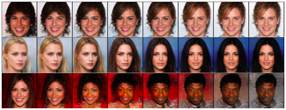
Below is a simple summary of the content related to the GLANN model.
Implicit Maximum Likelihood
The foundation of the entire GLANN method is "Implicit Maximum Likelihood Estimation," from the paper "Implicit Maximum Likelihood Estimation", referred to as "IMLE." This article was only posted on arXiv last September, which surprised me greatly. Because this algorithm is so simple, I had already used it two years ago. I always felt it was an obviously valid method, yet it was published so late... (I feel like I missed out on a fortune).
Directly Estimating Probability Distributions
The appendix of IMLE provides a long series of complex mathematical derivations, but I feel they are not strictly necessary. IMLE is essentially the result of an integral approximation of the Dirac distribution.
In general, consider the following sampling process: z\sim q(z),\quad x = G(z) This is equivalent to assuming the distribution of x is: q(x)=\int \delta\big(x-G(z)\big)q(z)dz where q(z) is generally a normal or uniform distribution, and \delta(\cdot) represents the (multivariate) Dirac delta function.
Note that q(x) can also be written as: q(x)=\mathbb{E}_{z\sim q(z)}\big[\delta\big(x-G(z)\big)\big] And \delta(\cdot) is actually a Gaussian distribution with variance tending to 0: \delta(x)=\lim_{\sigma\to 0}\frac{1}{(2\pi\sigma^2)^{d/2}}\exp\left(-\frac{\Vert x\Vert^2}{2\sigma^2}\right) Thus, we might as well let \sigma take a finite value, perform the calculation, and then let \sigma\to 0: q(x)=\lim_{\sigma\to 0}\mathbb{E}_{z\sim q(z)}\left[\frac{1}{(2\pi\sigma^2)^{d/2}}\exp\left(-\frac{\Vert x - G(z)\Vert^2}{2\sigma^2}\right)\right] Then, we perform maximum likelihood estimation, using -\int p(x)\log q(x)dx as the loss, where p(x) is the distribution of real samples: \begin{aligned} loss &= -\int p(x)\log \left\{\mathbb{E}_{z\sim q(z)}\left[\frac{1}{(2\pi\sigma^2)^{d/2}}\exp\left(-\frac{\Vert x - G(z)\Vert^2}{2\sigma^2}\right)\right]\right\}dx \\ &= \mathbb{E}_{x\sim p(x)}\left[-\log \left\{\mathbb{E}_{z\sim q(z)}\left[\frac{1}{(2\pi\sigma^2)^{d/2}}\exp\left(-\frac{\Vert x - G(z)\Vert^2}{2\sigma^2}\right)\right]\right\}\right] \\ &\sim \mathbb{E}_{x\sim p(x)}\left[-\log \left\{\mathbb{E}_{z\sim q(z)}\left[\exp\left(-\frac{\Vert x - G(z)\Vert^2}{2\sigma^2}\right)\right]\right\}\right] \end{aligned} In the last expression, we have omitted constants irrelevant to optimization.
Now we convert the expectation \mathbb{E} into sampling, substituting x_1,x_2,\dots,x_M\sim p(x) and z_1,z_2,\dots,z_N\sim q(z) into the loss: \begin{aligned} loss &\sim -\frac{1}{M}\sum_{i=1}^M \log \left\{\frac{1}{N}\sum_{j=1}^N\exp\left(-\frac{\Vert x_i - G(z_j)\Vert^2}{2\sigma^2}\right)\right\} \\ &\sim -\frac{1}{M}\sum_{i=1}^M \log \left\{\sum_{j=1}^N\exp\left(-\frac{\Vert x_i - G(z_j)\Vert^2}{2\sigma^2}\right)\right\} \end{aligned} As we know from the article "Seeking a Smooth Maximum Function", the \text{logsumexp} (exponentiate, sum, then take the logarithm) is actually a smooth approximation of the \max function. As \sigma\to 0, it becomes the \max. With the negative sign, it becomes the \min. Thus, the simplest form as \sigma\to 0 is: loss\sim \frac{1}{M}\sum_{i=1}^M \left(\min_{j=1}^N \Vert x_i - G(z_j)\Vert^2\right) This is the loss used by IMLE. (The derivation is a bit long only because it is detailed; it is not actually difficult.)
Therefore, in the specific workflow of IMLE:
1. Sample a batch of real samples x_1,x_2,\dots,x_M;
2. Sample a batch of noise z_1,z_2,\dots,z_N to obtain a batch of fake samples \hat{x}_1,\hat{x}_2,\dots,\hat{x}_N;
3. For each real sample x_i, find its nearest fake sample \hat{x}_{\rho(i)};
4. Minimize the average distance \frac{1}{M}\sum\limits_{i=1}^M \Vert x_i - \hat{x}_{\rho(i)}\Vert^2.
Effect Analysis and Discussion
Putting the derivation aside, this algorithm is very intuitive: If every real sample can find a sufficiently close match among the fake samples, doesn’t that mean the fake samples are generated quite well? This is why I said it’s unbelievable that this algorithm was published so late.
Now let’s look at the results. The principle of the algorithm is sound, but the problem is that the "nearest" search in the above algorithm uses the L_2 distance. For images, L_2 is not a good metric, so one can imagine this method suffers from the same blurriness issues as VAEs. In fact, looking at the results on CelebA, it doesn’t even match up to VAE:
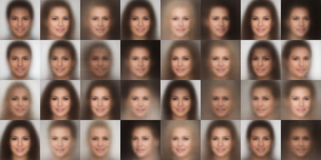
Code: https://github.com/bojone/gan/blob/master/imle.py
Actually, this idea can be extended to general divergence optimization. For example, we can use: KL(q(x)\Vert p(x))=\int q(x)\log \frac{q(x)}{p(x)}dx=\mathbb{E}_{x\sim q(x)}\big[\log q(x)-\log p(x)\big] as the optimization objective. Then, processing \log q(x) and \log p(x) in the same way, the result is: loss\sim -\frac{1}{M}\sum_{i=1}^M \left(\min_{j=1}^N \Vert G(z_i) - x_j\Vert^2 - \min_{j=1}^K \Vert G(z_i) - G(z_j)\Vert^2\right) Alternatively, setting a margin m can yield better results: loss\sim -\frac{1}{M}\sum_{i=1}^M \left(\min_{j=1}^N \Vert G(z_i) - x_j\Vert^2 + \text{relu}\left(m - \min_{j=1}^K \Vert G(z_i) - G(z_j)\Vert^2\right)\right) Note that two batches of fake samples must be sampled here; otherwise, the second term would be meaningless (within the same batch, the second term is always 0). The second term is used to prevent mode collapse. The workflow for this new algorithm is:
1. Sample a batch of real samples x_1,x_2,\dots,x_M;
2. Sample a batch of noise z_1,z_2,\dots,z_N to obtain a batch of fake samples \hat{x}_1,\hat{x}_2,\dots,\hat{x}_N;
3. Sample another batch of noise z_{N+1},z_{N+2},\dots,z_{N+K} to obtain another batch of fake samples \hat{x}_{N+1},\hat{x}_{N+2},\dots,\hat{x}_{N+K};
4. For each fake sample \hat{x}_i (1\leq i\leq N), find its nearest real sample x_{\rho_1(i)};
5. For each fake sample \hat{x}_i (1\leq i\leq N), find its nearest fake sample x_{N+\rho_2(i)} among \hat{x}_{N+1},\dots,\hat{x}_{N+K};
6. Minimize the "real-fake" distance while maximizing the "fake-fake" distance, i.e., the loss above.
Results:
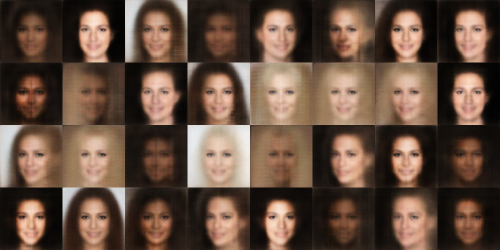
They are all quite similar...
From IMLE to GLANN
Returning to the discussion of IMLE itself, one can imagine that the main reason for its poor performance is the use of L_2 distance. So, what if we replace it with other distances? For image realism, are there existing loss functions we can use?
Perceptual Loss
There actually is one: perceptual loss! This perceptual loss originates from style transfer, likely from the paper "Perceptual Losses for Real-Time Style Transfer and Super-Resolution". Calculating this perceptual loss is somewhat complex; it requires a pre-trained ImageNet model (usually VGG). One calculates the L_2 (or L_1) distance of the last few hidden layer vectors and the L_2 (or L_1) distance of the Gram matrices, then sums them up.
This distance works well in style transfer tasks, but it is complex to compute and feels more like an engineering product than a result of theoretical derivation. Therefore, I don’t particularly like it and have no interest in writing about it in detail. In short, one can combine perceptual loss with IMLE: loss\sim \frac{1}{M}\sum_{i=1}^M \left(\min_{j=1}^N d_{perceptual}\big(x_i,G(z_j)\big)\right)\label{eq:perceptual-1}
Intermediate Product: GLO
Directly optimizing objective \eqref{eq:perceptual-1} is theoretically fine, but the computational cost is enormous. As mentioned, perceptual loss is complex to calculate and requires a pre-trained ImageNet model. If the batch size is 64, we would need to calculate 64^2=4096 perceptual losses per batch and then take the minimum, which would be unacceptably slow or even impossible to run.
Therefore, GLANN also utilizes a technique called GLO, from the paper "Optimizing the latent space of generative networks".
GLO is also an extremely simple concept that somehow became a full paper. GLO does not intend to be a generative model; it only aims to obtain a low-dimensional embedding. Assuming the real sample set is x_1,x_2,\dots,x_M, the optimization objective of GLO is: \mathop{\text{argmin}}_{G,\hat{z}_1,\dots,\hat{z}_M}\frac{1}{M}\sum_{i=1}^M d\big(x_i, G(\hat{z}_i)\big)\quad \text{s.t.}\quad \Vert z_i\Vert=1 GLO optimizes \hat{z}_1,\dots,\hat{z}_M directly, which is equivalent to an Embedding layer, training an embedding for each image. The parts of the model that can vary are the constraints on the Embedding and the metric d used. For GLANN, perceptual loss is used: \mathop{\text{argmin}}_{G,\hat{z}_1,\dots,\hat{z}_M}\frac{1}{M}\sum_{i=1}^M d_{perceptual}\big(x_i, G(\hat{z}_i)\big)\quad \text{s.t.}\quad \Vert z_i\Vert=1 This way, even with a batch size of 64, we only need to calculate 64 perceptual losses per batch because it does not involve pairwise comparisons.
Final Result: GLANN
Now that we have \hat{z}_1,\dots,\hat{z}_M, G(\hat{z}_i) can generate images. We only need to treat \hat{z}_1,\dots,\hat{z}_M as the "original images" and apply IMLE (at this point, L_2 can be used because it is in the latent space): \mathop{\text{argmin}}_{T}\frac{1}{M}\sum_{i=1}^M \left(\min_{j=1}^N \Vert \hat{z}_i - T(z_j)\Vert^2\right) This gives us the generative model. The complete generation process is: z\sim q(z)\quad\xrightarrow{\quad T\quad }\quad \hat{z}_i \quad \xrightarrow{\quad G\quad }\quad x_i
Personal Evaluation
At this point, we have finished explaining the GLANN model. Overall, it is a model that integrates several techniques. As for the results, just look at the images at the beginning; I actually think the results are not particularly good, as the backgrounds are always very messy. Of course, it is undoubtedly better than pure IMLE or GLO, and it should be much easier to train than a GAN.
The main improvement of GLANN is replacing the L_2 distance with perceptual loss. In fact, this replacement could likely be used in many models; I suspect it could also be applied to VAEs. On the other hand, the approach of perceptual loss is too engineering-oriented, which I find uninteresting, so I have no interest in researching it further. Additionally, the GLANN paper reports an advantage in FID on certain datasets. This looks good, but it is actually unfair. Since the calculation of FID itself relies on an ImageNet model, and GLANN’s loss also uses an ImageNet model, GLANN’s generation is naturally biased toward a better FID.
In fact, one could entirely use FID as a loss, train a GLO, and then train an IMLE to get a generative model. The FID of such a generative model would certainly be very low, but it would be meaningless because the realism of the images would not be guaranteed.
When reposting, please include the original address of this article: https://kexue.fm/archives/6394
For more detailed reposting matters, please refer to: "Scientific Space FAQ"